SPMD, communicators, point-to-point and collectives
Lars Pastewka
Learning objectives
After this lecture, you can
explain the SPMD model and the role of communicators, ranks and tags
write, compile and run a minimal MPI program
distinguish point-to-point from collective communication and avoid the classic send/send deadlock
estimate the cost of a reduction (naive vs tree) and explain why floating-point results may differ bit-wise
combine MPI with Kokkos, including GPU-aware MPI and mandatory fences
Why MPI?
Kokkos parallelizes within a node (shared memory / single GPU)
To use multiple nodes (distributed memory), we need message passing
MPI = Message Passing Interface, standardized since the 1990s
Each MPI process has its own separate address space
MPI is an abstraction layer: you don’t need to know the network topology, switches, or node configuration
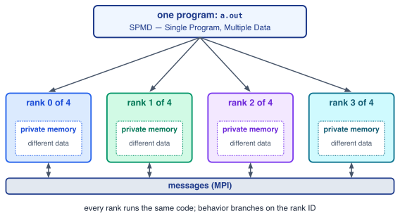
Single Program, Multiple Data (SPMD)
The same program runs on every process; each operates on a subset of the data.
Figure 1: One executable, launched as many ranks: each rank has its own private memory and operates on different data; ranks communicate only via the network.
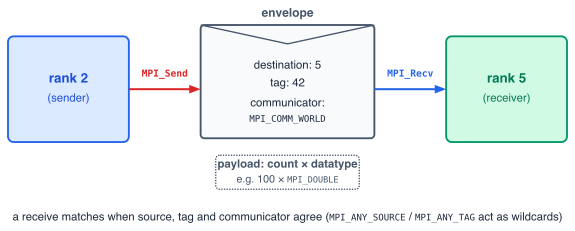
Figure 2: A message is a payload (count × datatype) plus an envelope: destination/source rank, tag and communicator. A receive matches a send only when all envelope fields agree.
Point-to-point: one sender, one receiver (Send/Recv/Sendrecv) – the envelope decides which receive matches which send
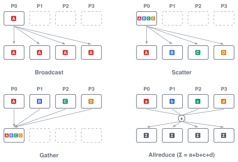
Collective: all processes participate (Bcast/Reduce/Scatter/Gather) – next slides
Communicators
All processes in an MPI program share the communicator MPI_COMM_WORLD.
#include <mpi.h>#include <stdio.h>int main(int argc,char** argv){ MPI_Init(&argc,&argv);int world_size, world_rank; MPI_Comm_size(MPI_COMM_WORLD,&world_size); MPI_Comm_rank(MPI_COMM_WORLD,&world_rank); printf("Hello from process %d of %d\n", world_rank, world_size); MPI_Finalize();return0;}
Figure 3: Bcast distributes one value to all; Scatter deals out pieces; Gather collects them; Allreduce combines values and gives everyone the result.
These four cover 90% of what you need; the full list is in the references (see Reading).
Point-to-point: requirements
For a Send/Recv pair to succeed:
Sender specifies a valid destination rank
Receiver specifies a valid source rank (or MPI_ANY_SOURCE)
The communicator is the same on both sides
Tags match (or receiver uses MPI_ANY_TAG)
Datatypes match
Receiver’s buffer is large enough
MPI_Send(buf, n, MPI_DOUBLE, dest, tag, MPI_COMM_WORLD);MPI_Recv(buf, n, MPI_DOUBLE, src, tag, MPI_COMM_WORLD,&status);
Blocking, non-blocking, combined
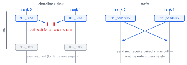
Blocking: MPI_Send/MPI_Recv – simple but easy to deadlock
Non-blocking: MPI_Isend/MPI_Irecv + MPI_Waitall – overlap communication with computation
Combined: MPI_Sendrecv – send and receive in one call, avoids deadlock by construction
The classic deadlock – and the fix
Figure 4: Two ranks that both MPI_Send first wait for each other forever. MPI_Sendrecv schedules the send and receive halves internally so matching pairs can never block each other.
MPI_Sendrecv(send_right, n, MPI_DOUBLE, right_neighbor, tag, recv_left, n, MPI_DOUBLE, left_neighbor, tag, MPI_COMM_WORLD,&status);
The standard deadlock-free tool for halo exchange (next lecture). MPI_PROC_NULL as partner turns either half into a no-op.
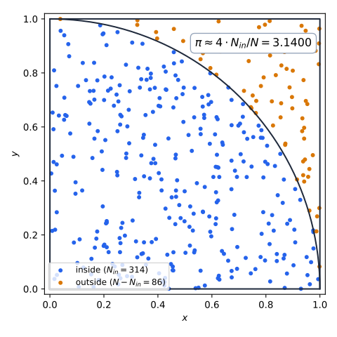
Independent part: evaluating \(\Theta(1 - (x_i^2 + y_i^2))\) per sample – no communication, embarrassingly parallel, distribute the \(N\) samples over \(s\) ranks
Reduction part: the sum \(\sum_i\) – this is where ranks must communicate
Almost every parallel program decomposes this way; the reduction is the part that costs.
Reduction cost
A reduction over \(s\) ranks combines \(d_0 \star d_1 \star \dots \star d_{s-1}\):
Naive: rank 0 receives and adds one partial result at a time → \(s - 1\) sequential communication steps
Tree: combine pairwise in rounds → \(\lceil \log_2 s \rceil\) steps – this is what MPI_Reduce does internally
For \(s = 1024\): 1023 steps vs. 10 steps.
Caveat: the tree changes the order of additions – and floating-point addition is not associative → results may differ bit-wise between runs and rank counts.
⇒ Different process counts may give bit-different results, even if mathematically the sum is the same.
GPU-aware MPI
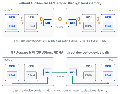
Figure 6: Without GPU-aware MPI, every message is staged through host memory on both sides. GPU-aware MPI sends directly from device memory (GPUDirect RDMA).
Kokkos::fence();MPI_Send(d_data.data(), N, MPI_DOUBLE, dest, tag, comm);
This works because of the Unified Virtual Address Space (UVA): host and device pointers live in the same numerical address range, so MPI can tell from a pointer where the data resides (UVA is not Unified Memory). 3–50× faster for large messages; requires a CUDA-/HIP-aware MPI build (e.g. mpi/openmpi/5.0-nvidia on bwUniCluster).
MPI + Kokkos: practical rules
int main(int argc,char* argv[]){ MPI_Init(&argc,&argv);// 1. MPI first Kokkos::initialize(argc, argv);// 2. then Kokkos/* ... your code ... */ Kokkos::finalize();// 3. Kokkos before MPI MPI_Finalize();return0;}
Initialize MPI before Kokkos, finalize in reverse order
Use the low-level C MPI interface, not C++ wrappers
Always call Kokkos::fence() before passing device pointers to MPI – GPU kernels are asynchronous and may still be running
Synchronization is mandatory
// WRONG: MPI may read stale dataKokkos::parallel_for("compute", N, kernel);MPI_Send(data.data(), N, MPI_DOUBLE,...);// CORRECT: fence before MPIKokkos::parallel_for("compute", N, kernel);Kokkos::fence();// wait for the GPUMPI_Send(data.data(), N, MPI_DOUBLE,...);