Scaling & Performance
Measuring strong/weak scaling, profiling, benchmarking
Learning objectives
After this lecture you can
design and run strong- and weak-scaling experiments for your LBM code
predict scaling limits with Amdahl’s and Gustafson’s laws
interpret a measured speedup curve (super-linear, plateau, rollover)
choose the right tool: profiler, microbenchmark, or scaling run
Milestone 6: a scaling plot of your code
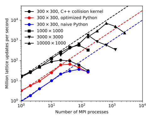
Million lattice updates per second vs. MPI processes for LBM implementations; Greiner & Pastewka, Proceedings of the bwHPC Symposium (2019).
This is the kind of plot you will produce – intuition alone is not reliable, you must measure .
Strong scaling
Fixed problem size, increase number of processes \(p\) :
\[S(p) = \frac{T_1}{T_p}, \qquad E(p) = \frac{S(p)}{p}\]
Plot \(S\) vs. \(p\) on log-log axes; ideal: slope = 1
Answers: how much faster can I solve this problem?
Deriving Amdahl’s law. Split the serial runtime \(T_1\) into a part that cannot be parallelized and a part that can:
\[T_1 = \underbrace{f_s\,T_1}_{\text{serial}} + \underbrace{(1-f_s)\,T_1}_{\text{parallelizable}}\]
On \(p\) processes the parallel part shrinks by \(p\) , the serial part is unchanged:
\[T_p = f_s\,T_1 + \frac{(1-f_s)\,T_1}{p}
\;\Rightarrow\;
S(p) = \frac{T_1}{T_p} = \frac{1}{f_s + \dfrac{1-f_s}{p}}
\;\xrightarrow{p\to\infty}\;
\frac{1}{f_s}\]
\(T_1\) : runtime on 1 process; \(T_p\) : runtime on \(p\) processes\(S(p)\) : speedup; \(E(p)\) : parallel efficiency; \(p\) : number of processes\(f_s\in[0,1]\) : serial (non-parallelizable) fraction; \(1-f_s\) : parallelizable fraction
Amdahl’s law
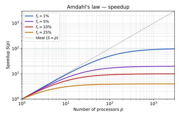
Amdahl’s law: a serial fraction \(f_s\) caps the speedup at \(S_\max = 1/f_s\) .
Even 1% serial code limits you to \(100\times\) – and communication overhead bites earlier.
Parallel efficiency
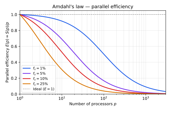
Strong-scaling efficiency \(E = S/p\) under Amdahl’s law: efficiency decays even before the speedup visibly saturates.
Report efficiency alongside speedup – it exposes waste that log-log speedup plots hide.
Weak scaling
Fixed work per process , increase \(p\) to solve a larger problem:
\[E(p) = \frac{T_1}{T_p} \qquad \text{(ideal: flat line at } 100\%\text{)}\]
Answers: can I solve a bigger problem? – often the more relevant question
Deriving Gustafson’s law. Measure the scaled workload on \(p\) processes and normalize its runtime to \(T_p = 1\) . Split it into a serial and a parallel part:
\[T_p = f_s' + (1-f_s') = 1\]
Re-running this same work on a single process leaves the serial part unchanged but expands the parallel part \(p\) -fold:
\[T_1 = f_s' + p\,(1-f_s')
\;\Rightarrow\;
S(p) = \frac{T_1}{T_p} = f_s' + p\,(1-f_s') = p - f_s'\,(p-1)\]
\(f_s'\in[0,1]\) : serial fraction of the scaled workload (measured on \(p\) processes, not on 1 as in Amdahl)\(1-f_s'\) : parallelizable fraction; \(p\) : number of processesSpeedup grows near-linearly in \(p\) when \(f_s'\) is small – no fixed ceiling
The metric: MLUPS
\[\text{MLUPS} = \frac{N_x \cdot N_y \cdot \text{timesteps}}{\text{wall time} \cdot 10^6}\]
M illion l attice u pdates p er s econd – the standard LBM throughput metricComparable across grid sizes, process counts, and machines
Report your milestone-6 performance in MLUPS
Running scaling experiments
Isolate the computation : time only the LBM loop, exclude I/O and initializationUse a dedicated cluster (bwUniCluster), not a laptopRun multiple times and report the median (variability is real)Vary \(p\) systematically : 1, 2, 4, 8, 16, 32, …Strong scaling: fixed grid; weak scaling: scale the grid with \(p\) (e.g. \(N_x \propto p\) )
Interpreting results
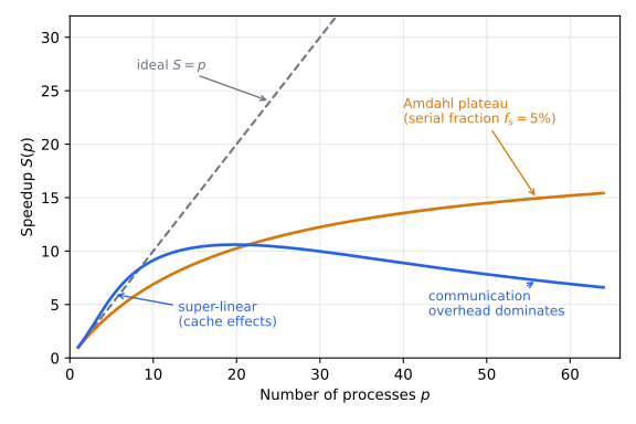
Four regimes: ideal (\(S = p\) ) → super-linear (local problem fits in cache) → Amdahl plateau (serial fraction) → rollover (communication overhead dominates).
Profiling with perf (CPU)
A profiler answers: where does the time go on one rank? (A scaling run answers: does the whole code scale.)
perf stat -e cache-references,cache-misses ./programperf record -g ./program && perf report -G Compile with -fno-omit-frame-pointer for accurate call stacks.
Key metrics: cache-misses, branch-misses, topdown-mem-bound.
GPU profiling
Kernel profiling answers: is each GPU kernel using the hardware well?
NVIDIA : ncu (Nsight Compute) per kernel, nsys (Nsight Systems) for the timeline
ncu --set full ./my_lbmnsys profile ./my_lbmAMD : rocprof
Key metrics: occupancy, memory throughput, achieved vs. peak bandwidth.
Microbenchmarking with Google Benchmark
A microbenchmark answers: how fast is this one function – and does a change make it faster?
static void BM_collision( benchmark:: State& state) { int N = state. range( 0 ); // setup ... for ( auto _ : state) { ( f, rho, u, omega); } . SetComplexityN( N); } ( BM_collision)-> Range( 64 , 4096 )-> Complexity();
Summary
Strong scaling: fixed problem, \(S(p) = T_1/T_p\) ; Amdahl caps it at \(1/f_s\)
Weak scaling: fixed work per process; Gustafson says big problems scale
Real curves show super-linear cache effects, then a plateau, then rollover
Measure MLUPS, isolate the compute loop, report medians
Profilers and microbenchmarks diagnose why ; scaling runs show whether