DGLs erster Ordnung

Differentialgleichungen – Kapitel 2

M. Ladecký, L. Pastewka

IMTEK, Universität Freiburg

Lernziele

Die Studierenden sollen…

• … das Richtungsfeld einer Differentialgleichung erster Ordnung interpretieren können.
• … die Methode der Separation der Variablen auf separierbare Differentialgleichungen anwenden können.
• … lineare Differentialgleichungen erster Ordnung mit der Methode des integrierenden Faktors lösen können.

Differentialgleichungen erster Ordnung

Allgemeine Form und Anfangswertproblem

• Beziehung zwischen gesuchter Funktion \(y(x)\) und ihrer ersten Ableitung:

\[ \frac{\mathrm{d}y}{\mathrm{d}x} = f(x, y) \]

• Die allgemeine Lösung ist eine Familie von Lösungen mit einer freien Integrationskonstanten
• Eine Anfangsbedingung \(y(x_0) = y_0\) wählt eine konkrete Lösung aus
• DGL + Anfangsbedingung = Anfangswertproblem

Das Richtungsfeld

• Geometrische Interpretation: \(f(x, y)\) gibt an jedem Punkt \((x, y)\) die Steigung der Lösungskurve an
• Gesamtheit aller Richtungspfeile = Richtungsfeld der DGL
• Eine Lösungskurve folgt dem Strömungsfeld: ihre Tangente stimmt überall mit dem Richtungspfeil überein
• Erlaubt qualitative Aussagen ohne explizite Lösung:
  • Wachsen oder fallen die Lösungen?
  • Streben sie gegen bestimmte Werte? Oszillieren sie?

Separation der Variablen

Die Methode

• Eine DGL heißt separabel, wenn die rechte Seite faktorisiert:

\[ \frac{\mathrm{d}y}{\mathrm{d}x} = g(x)\,h(y) \]

• Variablen trennen und beide Seiten unabhängig integrieren:

\[ \int \frac{1}{h(y)}\,\mathrm{d}y = \int g(x)\,\mathrm{d}x + C \]

• Führt die DGL auf zwei gewöhnliche Integrale zurück; Ergebnis: implizite oder explizite Gleichung für \(y(x)\)
• Grenzen: \(y' = x + y\) oder \(y' = x^2 + y^2\) sind nicht separabel; Nullstellen von \(h(y)\) definieren oft konstante Lösungen, die bei der Separation verloren gehen können

Lineare Differentialgleichungen erster Ordnung

Standardform

\[ \frac{\mathrm{d}y}{\mathrm{d}x} + p(x)\,y = q(x) \]

• Kennzeichen: \(y\) und \(y'\) treten nur in erster Potenz auf (keine Terme wie \(y^2\), \(\sin(y)\), \((y')^2\))
• \(p(x)\) und \(q(x)\) sind beliebige Funktionen von \(x\), dürfen aber nicht von \(y\) abhängen
• Homogen: \(q(x) = 0\) → separabel, durch Trennung der Variablen lösbar
• Inhomogen: \(q(x) \neq 0\) → spezielle Lösungsmethode nötig

Die Methode des integrierenden Faktors

• Idee: Multipliziere die Gleichung mit \(\mu(x)\), sodass die linke Seite zur Produktableitung \(\frac{\mathrm{d}}{\mathrm{d}x}[\mu(x)\,y]\) wird
• Koeffizientenvergleich mit der Produktregel liefert \(\mu'(x) = \mu(x)\,p(x)\), also (Integrationskonstante entbehrlich):

\[ \mu(x) = e^{\int p(x)\,\mathrm{d}x} \]

• Integration von \(\frac{\mathrm{d}}{\mathrm{d}x}[\mu(x)\,y] = \mu(x)\,q(x)\) und Auflösen nach \(y\):

\[ y(x) = \frac{1}{\mu(x)}\left[\int \mu(x)\,q(x)\,\mathrm{d}x + C\right] \]

• Funktioniert für jede lineare DGL erster Ordnung; reduziert das Problem auf zwei Integrationen

Existenz und Eindeutigkeit

Der Satz von Picard-Lindelöf

• Anfangswertproblem: \(y' = f(x, y)\), \(y(x_0) = y_0\)
• Satz: Sind \(f(x, y)\) und \(\partial f/\partial y\) in einer Umgebung von \((x_0, y_0)\) stetig, existiert eine eindeutige lokale Lösung
• Stetigkeit von \(f\) → Existenz; Stetigkeit von \(\partial f/\partial y\) (Lipschitz-Stetigkeit) → Eindeutigkeit
• Gegenbeispiel: \(y' = 2\sqrt{|y|}\), \(y(0) = 0\) hat unendlich viele Lösungen (\(\partial f/\partial y\) unstetig bei \(y = 0\))

Konsequenzen und Fortsetzbarkeit

• Eindeutigkeit: gleiche Anfangsbedingungen → gleiche zeitliche Entwicklung (keine Willkür)
• Existenz ist nur lokal garantiert; oft ist die Lösung jedoch über das Intervall hinaus fortsetzbar
• Blow-up: Lösung strebt in endlicher Zeit gegen unendlich, z.B. bei \(y' = y^2\) mit positivem Anfangswert – dort endet die maximale Fortsetzung
• Lineare DGLs mit stetigen Koeffizienten: Lösung existiert immer global – wichtige Vereinfachung gegenüber nichtlinearen Gleichungen

Beispiele

Exponentielles Wachstum und radioaktiver Zerfall

• Änderungsrate proportional zum aktuellen Wert → separable DGL:

\[ \frac{\mathrm{d}N}{\mathrm{d}t} = rN \qquad \Rightarrow \qquad N(t) = N_0\,e^{rt} \]

• Bakterienkultur (\(N_0 = 1000\), \(r = 0{,}5\)/h): \(N(3) = 1000\,e^{1{,}5} \approx 4482\)
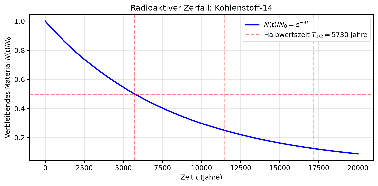
• \(r < 0\): exponentieller Zerfall, \(N(t) = N_0 e^{-\lambda t}\) mit Halbwertszeit

\[ \lambda = \frac{\ln 2}{T_{1/2}} \]

• Kohlenstoff-14 (\(T_{1/2} = 5730\) Jahre): nach 10000 Jahren noch \(\approx 0{,}3\,N_0\) vorhanden

Radioaktiver Zerfall: Visualisierung

Radioaktiver Zerfall von Kohlenstoff-14

Beispiel: Freier Fall mit Luftwiderstand

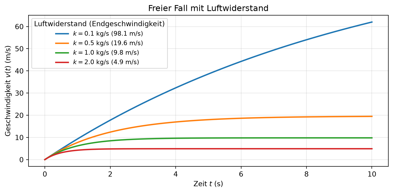
• Kräfte: Gewichtskraft \(mg\), Luftwiderstand \(-kv\) (proportional zur Geschwindigkeit)
• Inhomogene lineare DGL, Lösung mit integrierendem Faktor \(\mu(t) = e^{\frac{k}{m}t}\):

\[ m\frac{\mathrm{d}v}{\mathrm{d}t} = mg - kv \qquad \Rightarrow \qquad v(t) = \frac{mg}{k}\left(1 - e^{-\frac{k}{m}t}\right) \]

• Endgeschwindigkeit (Luftwiderstand kompensiert die Gewichtskraft):

\[ v_\infty = \lim_{t\to\infty} v(t) = \frac{mg}{k} \]

Freier Fall: Visualisierung

Fallende Objekte mit verschiedenen Luftwiderstandskoeffizienten

Beispiel: Mischungsproblem

• Tank: 100 L Wasser mit 20 kg Salz; Zufluss 0,5 kg/L mit 4 L/min, Abfluss 4 L/min (gut durchmischt)
• Bilanz: \(\dot{S} = \text{Einstrom} - \text{Ausstrom}\), lineare DGL:

\[ \frac{\mathrm{d}S}{\mathrm{d}t} = 2 - \frac{S}{25}, \quad S(0) = 20 \qquad \Rightarrow \qquad S(t) = 50 - 30\,e^{-t/25} \]

• Nach 30 Minuten: \(S(30) \approx 41\) kg
• Gleichgewicht \(S_\mathrm{eq} = 50\) kg: Konzentration im Tank = Zuflusskonzentration; charakteristische Zeit \(\tau = 25\) min

Beispiel: RC-Schaltkreis

• Widerstand \(R\) und Kondensator \(C\) in Reihe an Spannungsquelle \(V_0\); Kondensator anfangs ungeladen
• Kirchhoffsches Spannungsgesetz führt auf eine lineare DGL:

\[ \frac{\mathrm{d}V_\mathrm{C}}{\mathrm{d}t} + \frac{1}{RC}V_\mathrm{C} = \frac{V_0}{RC} \qquad \Rightarrow \qquad V_\mathrm{C}(t) = V_0\left(1 - e^{-\frac{t}{RC}}\right) \]

• Zeitkonstante \(\tau = RC\): nach \(\tau\) sind \(\approx 63\,\%\) des Endwerts erreicht, nach \(\approx 5\tau\) ist der Kondensator praktisch voll geladen
• Große Werte von \(R\) oder \(C\) → langsamer Ladevorgang; fundamentale Rolle für Zeitverzögerungen und Filter in der Elektronik

Zusammenfassung

• DGL erster Ordnung \(y' = f(x, y)\): allgemeine Lösung = Lösungsfamilie, Anfangsbedingung wählt eine Lösung aus; das Richtungsfeld liefert qualitative Einsicht
• Separation der Variablen für \(y' = g(x)h(y)\): führt auf zwei unabhängige Integrationen
• Integrierender Faktor \(\mu(x) = e^{\int p\,\mathrm{d}x}\) löst jede lineare DGL erster Ordnung systematisch
• Picard-Lindelöf: Stetigkeit von \(f\) und \(\partial f/\partial y\) garantiert eindeutige lokale Lösung
• Anwendungen: Wachstum/Zerfall, freier Fall, Mischung, RC-Schaltkreis – alle zeigen exponentielle Annäherung an Grenzwerte