Funktionenräume und Basis-Entwicklungen
Differentialgleichungen – Kapitel 8
M. Ladecký, L. Pastewka
IMTEK, Universität Freiburg
Lernziele
Die Studierenden sollen…
- … das innere Produkt von Funktionen erklären und Orthogonalität von Basisfunktionen nachweisen können.
- … Fourier-Koeffizienten für periodische Funktionen berechnen und Fourier-Reihen aufstellen können.
- … die Fourier-Transformation auf nicht-periodische Funktionen anwenden und deren Eigenschaften nutzen können.
Von Vektoren zu Funktionen
- Eine Funktion besitzt an jedem Punkt eines Intervalls einen Wert – wie ein Vektor mit unendlich vielen Komponenten
- Endlich-dimensional: jeder Vektor ist Linearkombination von Basisvektoren
\[ \mathbf{a} = a_1 \mathbf{e}_1 + a_2 \mathbf{e}_2 + a_3 \mathbf{e}_3 \]
- Zentrale Frage: Können Funktionen ebenfalls als Basis-Entwicklung geschrieben werden?
- Antwort: Ja – im unendlich-dimensionalen Funktionenraum übernehmen Funktionen die Rolle der Basisvektoren
Inneres Produkt und Norm
- Verallgemeinerung des Skalarprodukts \(\mathbf{a} \cdot \mathbf{b} = \sum_i a_i b_i\): Summe → Integral
\[ \langle f, g \rangle = \int_a^b f^*(x)\, g(x) \, dx \]
- Stern: komplexe Konjugation (für reelle Funktionen ohne Bedeutung)
- Norm = „Länge” einer Funktion:
\[ \|f\| = \sqrt{\langle f, f \rangle} = \sqrt{\int_a^b |f(x)|^2 \, dx} \]
- Quadrat der Norm entspricht physikalisch oft Energie oder Leistung
Orthogonalität
- Zwei Funktionen heißen orthogonal, wenn ihr inneres Produkt verschwindet:
\[ \langle f, g \rangle = 0 \]
- Geometrische Bedeutung: die Funktionen sind in keiner Weise miteinander korreliert
- Orthogonalität ist fundamental für die Konstruktion von Basisfunktionen
Basisfunktionen
- Eine Basis \(\{\varphi_n(x)\}_{n=1}^{\infty}\) muss linear unabhängig und vollständig sein
- Jede Funktion des Raums ist als unendliche Reihe darstellbar:
\[ f(x) = \sum_{n=1}^{\infty} a_n \varphi_n(x) \]
- Die Koeffizienten \(a_n\) spielen die Rolle der Vektorkomponenten
- Besonders nützlich: orthogonale Basisfunktionen mit
\[ \langle \varphi_m, \varphi_n \rangle = c_n \delta_{mn} \]
Koeffizienten und Parsevalsche Gleichung
- Bei orthogonaler Basis: Koeffizienten durch Projektion (inneres Produkt)
\[ a_n = \frac{\langle \varphi_n, f \rangle}{\langle \varphi_n, \varphi_n \rangle} = \frac{\langle \varphi_n, f \rangle}{c_n} \]
- Parsevalsche Gleichung – Energieerhaltung bei der Entwicklung:
\[ \langle f, f \rangle = \sum_{n=1}^{\infty} |a_n|^2 c_n \]
- Jeder Term \(|a_n|^2 c_n\) ist der Beitrag der \(n\)-ten Basisfunktion zur Gesamtenergie
Die Fourier-Basis
- Wichtigste Basis für periodische Funktionen (Periode \(L\)):
\[ \varphi_n(x) = e^{i 2\pi n x / L}, \quad n \in \mathbb{Z} \]
- Orthogonal über eine Periode:
\[ \langle \varphi_m, \varphi_n \rangle = L\, \delta_{mn} \]
- Reelle Form über Sinus- und Kosinus-Funktionen, z.B. \(\int_0^L \cos\!\left(\frac{2\pi m x}{L}\right)\cos\!\left(\frac{2\pi n x}{L}\right) dx = \frac{L}{2}\delta_{mn}\) für \(m, n \neq 0\)
Eigenfunktionen des Ableitungsoperators
- Die Fourier-Basis diagonalisiert den Ableitungsoperator:
\[ \frac{d}{dx} e^{i\omega x} = i\omega \cdot e^{i\omega x} \]
- \(e^{i\omega x}\) ist Eigenfunktion, \(i\omega\) der zugehörige Eigenwert
- Erklärt den Erfolg des Exponentialansatzes \(y = e^{\lambda t}\) (Kapitel 2):
\[ (a_n \lambda^n + a_{n-1}\lambda^{n-1} + \cdots + a_0)\, e^{\lambda t} = 0 \]
- Ableitungen werden zu Multiplikationen → DGL wird algebraische Gleichung
Fourier-Reihen (komplexe Form)
- Jede periodische Funktion mit Periode \(L\):
\[ f(x) = \sum_{n=-\infty}^{\infty} c_n e^{i 2\pi n x / L} \]
- Koeffizienten aus der Orthogonalitätsrelation:
\[ c_m = \frac{1}{L} \int_0^L f(x)\, e^{-i 2\pi m x / L} \, dx \]
- \(c_m\) misst den Anteil der Frequenz \(m \cdot 2\pi/L\) in der Funktion
Fourier-Reihen (reelle Form)
\[ f(x) = \frac{a_0}{2} + \sum_{n=1}^{\infty} \left[a_n \cos\left(\frac{2\pi n x}{L}\right) + b_n \sin\left(\frac{2\pi n x}{L}\right)\right] \]
mit den Koeffizienten
\[ a_n = \frac{2}{L} \int_0^L f(x) \cos\left(\frac{2\pi n x}{L}\right) dx, \quad b_n = \frac{2}{L} \int_0^L f(x) \sin\left(\frac{2\pi n x}{L}\right) dx \]
- Besonders geeignet für gerade/ungerade Funktionen: jeweils eine Reihe verschwindet
Fourier-Transformation
- Für nicht-periodische Funktionen: diskrete → kontinuierliche Frequenzvariable
\[ \hat{f}(k) = \mathcal{F}[f](k) = \int_{-\infty}^{\infty} f(x)\, e^{-ikx} \, dx \]
- Inverse Transformation rekonstruiert die ursprüngliche Funktion:
\[ f(x) = \mathcal{F}^{-1}[\hat{f}](x) = \frac{1}{2\pi} \int_{-\infty}^{\infty} \hat{f}(k)\, e^{ikx} \, dk \]
- \(\hat{f}(k)\) gibt die Amplitude der Frequenzkomponente \(k\) an
Differentiation im Fourier-Raum
- Wichtigste Eigenschaft für DGLs: Ableitung → Multiplikation
\[ \mathcal{F}\left[\frac{df}{dx}\right](k) = ik\, \hat{f}(k), \qquad \mathcal{F}\left[\frac{d^2f}{dx^2}\right](k) = -k^2\, \hat{f}(k) \]
- Differentialgleichungen mit konstanten Koeffizienten werden im Fourier-Raum zu algebraischen Gleichungen
- Grundlage der Fourier-Methoden zur Lösung von DGLs (Kapitel 9)
Wichtige Transformationspaare
| \(f(t)\) | \(\hat{f}(\omega)\) |
|---|---|
| \(\delta(t)\) | \(1\) |
| \(1\) | \(2\pi\delta(\omega)\) |
| \(e^{i\omega_0 t}\) | \(2\pi\delta(\omega - \omega_0)\) |
| \(\cos(\omega_0 t)\) | \(\pi[\delta(\omega - \omega_0) + \delta(\omega + \omega_0)]\) |
| \(e^{-a|t|}\) \((a > 0)\) | \(\frac{2a}{a^2 + \omega^2}\) |
| \(e^{-at}\Theta(t)\) \((a > 0)\) | \(\frac{1}{a + i\omega}\) |
| \(\text{rect}(t/T)\) | \(T \cdot \text{sinc}(\omega T/2)\) |
| \(e^{-t^2/(2\sigma^2)}\) | \(\sigma\sqrt{2\pi}\, e^{-\omega^2\sigma^2/2}\) |
Wichtige Rechenregeln
| Eigenschaft | Zeitbereich | Frequenzbereich |
|---|---|---|
| Linearität | \(\alpha f(t) + \beta g(t)\) | \(\alpha\hat{f}(\omega) + \beta\hat{g}(\omega)\) |
| Zeitverschiebung | \(f(t - t_0)\) | \(e^{-i\omega t_0}\hat{f}(\omega)\) |
| Frequenzverschiebung | \(e^{i\omega_0 t}f(t)\) | \(\hat{f}(\omega - \omega_0)\) |
| Zeitskalierung | \(f(at)\) | \(\frac{1}{|a|}\hat{f}(\omega/a)\) |
| Differentiation | \(\frac{d^n f}{dt^n}\) | \((i\omega)^n\hat{f}(\omega)\) |
| Faltung | \((f * g)(t)\) | \(\hat{f}(\omega)\cdot\hat{g}(\omega)\) |
| Multiplikation | \(f(t)\cdot g(t)\) | \(\frac{1}{2\pi}(\hat{f} * \hat{g})(\omega)\) |
Das Faltungstheorem
- Faltung zweier Funktionen:
\[ (f * g)(x) = \int_{-\infty}^{\infty} f(x-y)\, g(y) \, dy \]
- Die Fourier-Transformierte der Faltung ist das Produkt der Transformierten:
\[ \mathcal{F}[f * g](k) = \hat{f}(k) \cdot \hat{g}(k) \]
- Für periodische Funktionen analog: \(c_n^{(f \circledast g)} = c_n^{(f)} \cdot c_n^{(g)}\)
- Anwendungen: Signalverarbeitung, Integralgleichungen, lineare Systemtheorie
Beispiel: Rechteckwelle
- Periodische Rechteckwelle (Periode \(L\), Amplitude \(A\)) mit Unstetigkeiten:
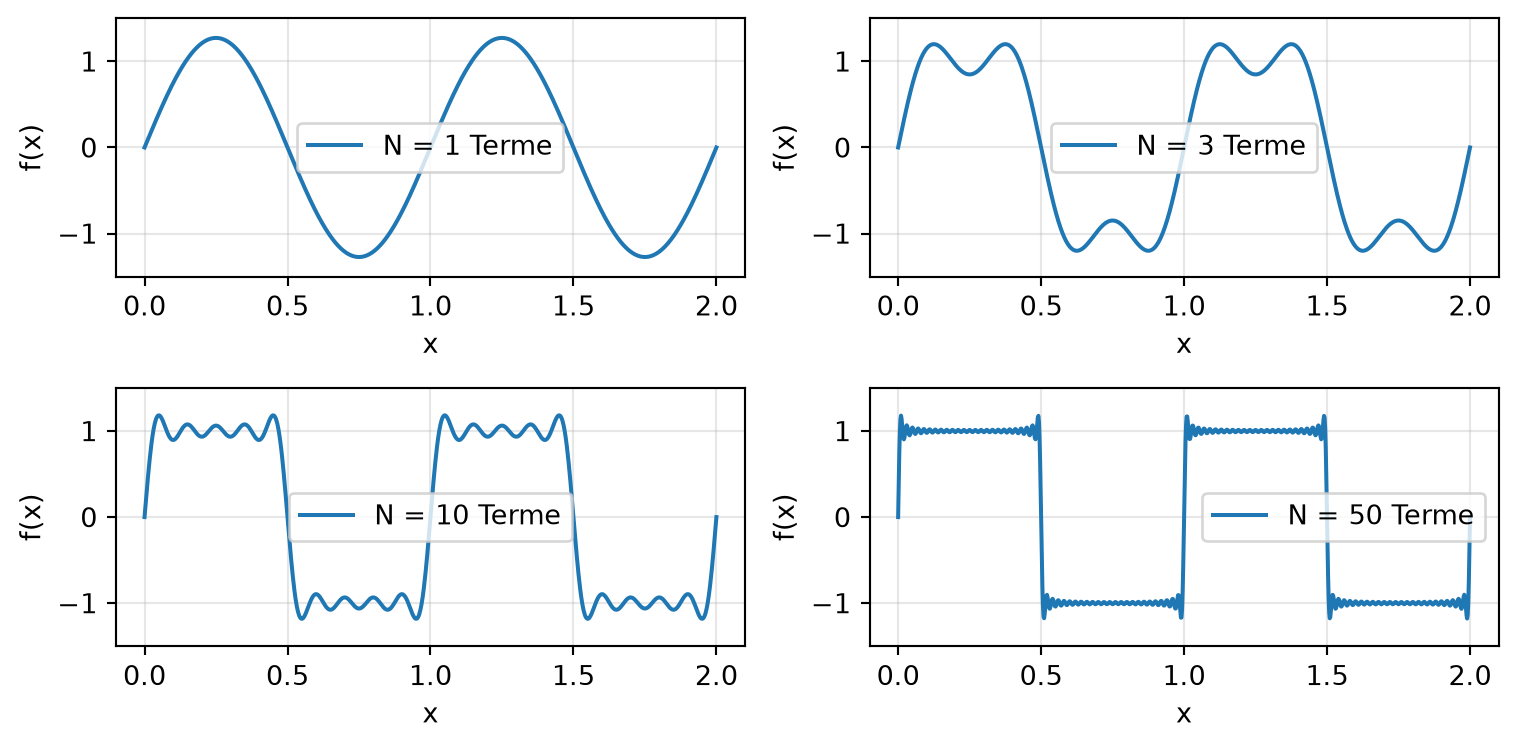
\[ f(x) = \frac{4A}{\pi}\sum_{n=1,3,5,\ldots}^{\infty} \frac{1}{n}\sin\left(\frac{2\pi n x}{L}\right) \]
- Nur ungerade Harmonische tragen bei
- Koeffizienten fallen mit \(1/n\) ab – Folge der Unstetigkeiten
- An den Sprungstellen: Gibbs-Phänomen (Überschwingen, das auch bei beliebig vielen Termen nicht verschwindet)
Beispiel: Konvergenz der Fourier-Reihe
Mit zunehmender Termzahl nähert sich die Reihe der Rechteckwelle; das Gibbs-Phänomen bleibt an den Sprungstellen sichtbar.
Beispiel: Fast Fourier Transform (FFT)
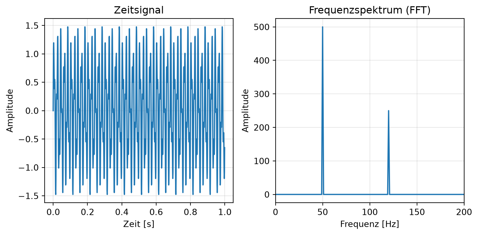
Die FFT (\(O(N \log N)\) statt \(O(N^2)\)) macht die Frequenzkomponenten bei 50 Hz und 120 Hz unmittelbar sichtbar.
Zusammenfassung
- Funktionen sind Elemente eines unendlich-dimensionalen Vektorraums; das innere Produkt \(\langle f, g \rangle = \int f^* g \, dx\) verallgemeinert das Skalarprodukt
- Orthogonale Basen erlauben Reihenentwicklungen mit einfach berechenbaren Koeffizienten; die Parsevalsche Gleichung drückt Energieerhaltung aus
- Die Fourier-Basis \(e^{i 2\pi n x/L}\) diagonalisiert den Ableitungsoperator – Eigenfunktionen mit Eigenwert \(i\omega\)
- Fourier-Reihen für periodische, Fourier-Transformation für nicht-periodische Funktionen
- Differentiation wird im Fourier-Raum zur Multiplikation mit \((i\omega)^n\) – Schlüssel zur Lösung linearer DGLs
Differentialgleichungen