Domain decomposition

Ghost cells, halo exchange, virtual topologies

Lars Pastewka

Learning objectives

After this lecture, you can

decompose a stencil-based solver into subdomains with ghost cells
implement a deadlock-free halo exchange with MPI_Sendrecv
handle corners in 2D/3D with the two-sweep trick
set up a Cartesian communicator and let MPI find your neighbours
choose between 1D strips and 2D tiles based on communication volume

The pattern: split the grid across ranks

Most stencil-based solvers (diffusion, wave equation, lattice Boltzmann) are nearest-neighbour. Each process owns a subdomain plus a layer of ghost cells that mirror its neighbour’s data.

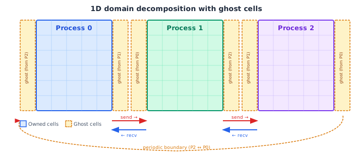
After every time step, ranks exchange the boundary layer – the halo exchange.

Worked example: 1D diffusion

A finite-difference discretization of the 1D diffusion equation:

\[ c_i(t + \Delta t) = c_i(t) + \frac{\Delta t \, D}{\Delta x^2} \big(c_{i-1} + c_{i+1} - 2 c_i\big) \]

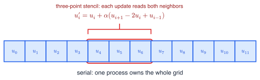
Figure 1: Serial baseline: one process owns the whole grid. The highlighted three-point stencil shows that each update reads both neighbours.

Distributing the grid across ranks

Spread \(N\) data points over \(s\) MPI processes. Process of rank \(r\) owns indices \(rN/s\) through \((r{+}1)N/s - 1\), plus one ghost cell on each side.

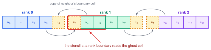
Figure 2: Ghost cells (dashed, amber) hold copies of the neighbouring rank’s edge cells; the highlighted stencil shows why the boundary update needs them.

Halo exchange with `Sendrecv`

# Python-style pseudocode -- C MPI is analogous
MPI.Sendrecv(
    sendbuf=c[-2],    # second-to-last interior cell (to right neighbour)
    dest=r+1,
    recvbuf=c[0],     # left ghost cell (from left neighbour)
    source=r-1)

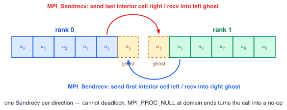
Figure 3: Each rank sends its last interior cell to the right neighbour’s ghost while receiving into its own left ghost – Sendrecv pairs both halves, avoiding deadlock.

For periodic boundary conditions, the first and last process exchange with each other (rank 0 ↔︎ rank \(s{-}1\)).

Ghost cells in 2D: lattice Boltzmann

The same idea, generalized to 2D and to a vector of populations \(f_{i,kl}\) at each lattice site:

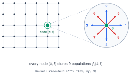
Figure 4: The D2Q9 lattice: every node \((k, l)\) stores nine populations \(f_0 \dots f_8\) – one rest population, four axis-aligned, four diagonal.

2D decomposition: who exchanges with whom?

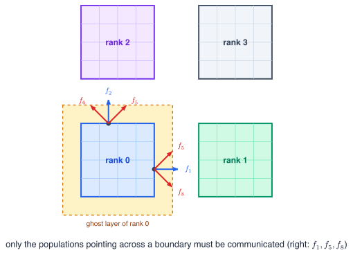
Figure 5: Each rank owns a tile plus a one-cell ghost frame (dashed). Only populations pointing across a boundary must be communicated: \(f_1, f_5, f_8\) cross the right edge (to rank 1), \(f_2, f_5, f_6\) the top edge (to rank 2). The diagonal populations land in the corners.

Corner exchange: do two sweeps

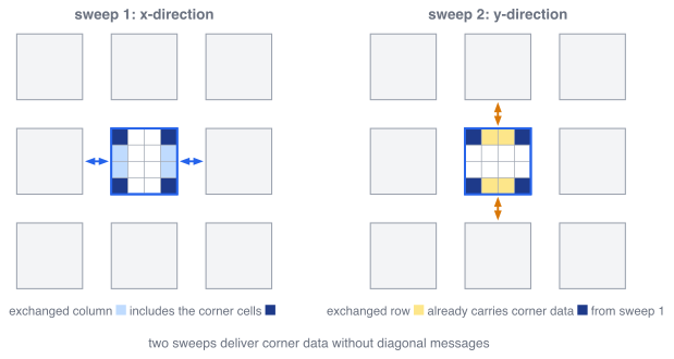
Figure 6: Sweep 1 exchanges in \(x\) (columns, including corners); sweep 2 exchanges in \(y\) (rows, which now carry the corner data). No diagonal message needed.

This is the standard trick for stencil halo exchange.

Virtual topologies: who is “left” and “right”?

In 2D and 3D, computing neighbour ranks by hand is error-prone. MPI provides a Cartesian communicator:

int dims[2] = {nx, ny};
int periods[2] = {1, 1};   // periodic in both directions
MPI_Comm cart;
MPI_Cart_create(MPI_COMM_WORLD, 2, dims, periods, /*reorder*/0, &cart);

int left, right;
MPI_Cart_shift(cart, /*direction*/0, /*disp*/1, &left, &right);

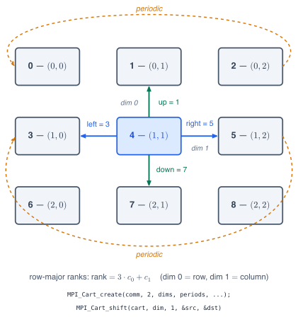
Figure 7: A 3×3 periodic Cartesian topology: each rank gets grid coordinates, and MPI_Cart_shift returns the neighbour ranks of (here) rank 4 in each direction – including the periodic wrap-around.

Choosing the decomposition shape

For \(s\) processes and an \(L \times L\) grid:

1D strips (\(s \times 1\)): boundary length \(L\), each strip’s halo is \(\propto L\)
2D tiles (\(\sqrt{s} \times \sqrt{s}\)): each tile’s halo is \(\propto L/\sqrt{s} \cdot 4\)

The 2D tiling has smaller communication volume per rank when \(s\) is large – but is more complex (corner exchange).

MPI_Dims_create will pick a balanced factorization for you.

The same idea generalizes to 3D – each rank owns a box and exchanges six faces.

Pitfalls and tips

Don’t forget the corners in 2D/3D (or use the two-sweep trick)
Always use Sendrecv for halo exchange – never Send then Recv in lockstep across ranks (deadlock risk)
Periodic BCs: the rank-0 ↔︎ rank-\((s{-}1)\) exchange is just another Sendrecv if you used a periodic Cartesian communicator
GPU-aware MPI: with the right MPI build you can Sendrecv directly on Kokkos device views (after Kokkos::fence())
Load balance: if \(N\) does not divide evenly by \(s\), distribute the remainder one cell per rank rather than dumping it on the last one