Domain decomposition

This chapter explains how to split a grid-based solver across multiple MPI processes. The MPI lecture introduced the message-passing machinery – ranks, point-to-point communication, collectives; here we use that machinery to parallelize stencil-based solvers such as the diffusion equation, the wave equation and the lattice Boltzmann method.

After working through this chapter, you can

• decompose a stencil-based solver into subdomains with ghost cells,
• implement a deadlock-free halo exchange with MPI_Sendrecv,
• identify which lattice Boltzmann populations must be communicated across each boundary,
• handle corners in a 2D decomposition with the two-sweep trick,
• set up a Cartesian communicator and let MPI compute your neighbors,
• choose between 1D strips and 2D tiles based on communication volume.

Why decompose?

A single GPU bounds your simulation in two ways. Its memory limits the lattice size: a 2D D2Q9 lattice stores nine double-precision populations per node, so a \(40{,}000 \times 40{,}000\) grid already needs more than 100 GB – beyond any single accelerator. Its throughput limits how fast you can advance even a lattice that fits: once a kernel saturates the memory bandwidth of the device, the only way to compute faster is to use more devices.

The remedy is domain decomposition: cut the grid into patches and give each MPI rank one patch. Every rank runs the same solver code on its own piece of the domain – this is the SPMD (single program, multiple data) model from the MPI lecture. The physics is local: stencil updates only read nearest neighbors, so ranks only need to talk to the ranks owning adjacent patches, and the data they exchange is a thin boundary layer. Compute scales with the patch area while communication scales with the patch perimeter, which is why this approach scales to thousands of GPUs.

The rest of this chapter develops the idea from a minimal 1D example to the full 2D lattice Boltzmann setting of milestone 6. For the mechanics of sending the messages themselves – MPI_Sendrecv, non-blocking communication, GPU-aware MPI – refer back to the MPI lecture.

A worked example in 1D: the diffusion equation

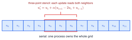
Consider the 1D diffusion equation \(\partial_t u = D \, \partial_x^2 u\), discretized with finite differences. With \(\alpha = D \Delta t / \Delta x^2\), one explicit time step updates every grid point from its two neighbors: \[ u_i' = u_i + \alpha \left( u_{i+1} - 2 u_i + u_{i-1} \right). \tag{1}\]

This is a three-point stencil: the new value at point \(i\) reads the old values at \(i-1\), \(i\) and \(i+1\). In a serial code, one process owns the whole grid and Equation 1 is a single loop (Figure 1).

Figure 1: The serial baseline: one process owns the entire 1D grid. The highlighted three-point stencil shows that each update reads both neighbors.

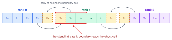
Now distribute the \(N\) grid points over \(s\) ranks, each owning a contiguous block of roughly \(N/s\) points. The stencil immediately raises a problem: to update its first point, a rank needs the last point of its left neighbor, which lives in a different address space.

When a grid is distributed across processes, each process owns a contiguous strip of grid points. To evaluate a finite-difference stencil at the edge of its strip, a process needs values of points owned by its neighbors. These are stored in ghost cells (also called halo cells): an extra layer of points on each side of the local domain that holds copies of the neighbors’ boundary data. Before each time step, the ghost cells are refreshed by a halo exchange: each process sends its outermost interior points to its neighbors and receives their boundary values in return.

Figure 2 shows the decomposed grid with its ghost cells, and Figure 3 shows the halo exchange that fills them.

Figure 2: The same 1D grid distributed over ranks. Each rank stores its interior points plus one ghost cell (dashed) on each side, holding a copy of the neighboring rank’s boundary cell. The highlighted stencil shows why the update of the first interior point needs the ghost value.

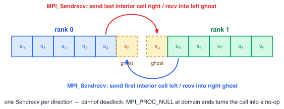
Figure 3: Halo exchange with MPI_Sendrecv: each rank sends its last interior cell to the right neighbor’s left ghost cell while receiving into its own left ghost cell, and vice versa for the other direction. Pairing each send with a receive in a single call avoids deadlock.

Putting it into code: a distributed wave solver

The following complete program implements exactly this picture for a closely related stencil, the 1D wave equation (acceleration \(a_i = (u_{i+1} - 2u_i + u_{i-1})/\Delta x^2\) – the same three-point pattern as Equation 1). It combines MPI for the halo exchange with Kokkos for the local stencil update, so it is also a template for how the two libraries interact in your own solver.

Each process stores n_local + 2 points: the interior points are at indices 1 to n_local, and the ghost cells sit at indices 0 and n_local + 1. The halo exchange uses MPI_Sendrecv (see the MPI lecture), which cannot deadlock, and MPI_PROC_NULL for the missing neighbors at the domain boundaries.

#include <mpi.h>
#include <Kokkos_Core.hpp>
#include <iostream>

using Field = Kokkos::View<double*>;

// Compute local part of wave equation.
// Interior points are at indices 1..n_local; ghosts at 0 and n_local+1.
void compute_wave_step(Field& u, Field& v, Field& a, int n_local, double dx, double dt) {
  // Acceleration on all interior points (the stencil reads the ghost cells)
  Kokkos::parallel_for(n_local, KOKKOS_LAMBDA(int i) {
    a(i + 1) = (u(i) - 2*u(i+1) + u(i+2)) / (dx * dx);
  });

  // Update velocity and displacement on the interior points
  Kokkos::parallel_for(n_local, KOKKOS_LAMBDA(int i) {
    v(i + 1) += a(i + 1) * dt;
    u(i + 1) += v(i + 1) * dt;
  });
  Kokkos::fence();  // Make kernel writes visible before the next halo exchange
}

int main(int argc, char* argv[]) {
  MPI_Init(&argc, &argv);
  Kokkos::initialize(argc, argv);

  {
    int rank, size;
    MPI_Comm_rank(MPI_COMM_WORLD, &rank);
    MPI_Comm_size(MPI_COMM_WORLD, &size);

    // Local domain size; see the domain decomposition diagrams above
    int n_local = 1000;

    Field u("u", n_local + 2);   // +2 for ghost cells at 0 and n_local+1
    Field v("v", n_local + 2);
    Field a("a", n_local + 2);

    // Neighbor ranks; MPI_PROC_NULL turns the exchange into a no-op
    int left = (rank > 0) ? rank - 1 : MPI_PROC_NULL;
    int right = (rank < size - 1) ? rank + 1 : MPI_PROC_NULL;

    // Simulate multiple time steps
    for (int step = 0; step < 100; ++step) {
      // Halo exchange: refresh ghost cells before computing
      // Send first interior point left, receive right ghost from the right
      MPI_Sendrecv(u.data() + 1, 1, MPI_DOUBLE, left, 0,
                   u.data() + n_local + 1, 1, MPI_DOUBLE, right, 0,
                   MPI_COMM_WORLD, MPI_STATUS_IGNORE);
      // Send last interior point right, receive left ghost from the left
      MPI_Sendrecv(u.data() + n_local, 1, MPI_DOUBLE, right, 1,
                   u.data(), 1, MPI_DOUBLE, left, 1,
                   MPI_COMM_WORLD, MPI_STATUS_IGNORE);

      // Compute locally
      compute_wave_step(u, v, a, n_local, 0.01, 0.001);
    }

    if (rank == 0) {
      std::cout << "Simulation complete" << std::endl;
    }
  }

  Kokkos::finalize();
  MPI_Finalize();
  return 0;
}

Note the structure of the time loop: exchange halos, then compute. Every parallel stencil solver – including your lattice Boltzmann code – has this same skeleton. This example fixes the boundary values at the ends of the global domain (via MPI_PROC_NULL); for periodic boundary conditions, rank \(0\) and rank \(s-1\) would instead exchange ghost data with each other.

Decomposing a 2D domain: strips

The simplest way to decompose a 2D grid is to keep the 1D decomposition logic and cut the domain along one axis only, into vertical (or horizontal) strips. Each rank then owns all rows of a contiguous range of columns, padded by one ghost column on each side, and exchanges halos with exactly two neighbors – precisely the pattern of the wave solver above, except that each message now carries a whole column instead of a single value.

Figure 4: A 2D grid decomposed into strips: each rank owns a contiguous block of columns plus one layer of ghost cells (dashed) on each side, populated by data received from the neighboring ranks. With periodic boundary conditions, the first and last ranks exchange ghost data with each other.

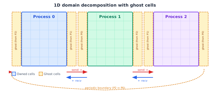
A strip decomposition is the most direct route to a working parallel lattice Boltzmann code, and it is the recommended starting point for milestone 6: two neighbors, two MPI_Sendrecv calls per exchange, no corner cases. We will return to its scaling limits below.

Domain decomposition for lattice Boltzmann

In the lattice Boltzmann method, the quantity living on the grid is not a single scalar but the nine populations of the D2Q9 velocity set: every node \((k, l)\) stores \(f_i(k, l)\) for \(i = 0, \dots, 8\) (Figure 5). In Kokkos this is naturally a three-dimensional view, e.g. Kokkos::View<double***> f("f", 9, nx, ny).

Figure 5: The D2Q9 data structure: every lattice node \((k, l)\) stores nine populations \(f_0, \dots, f_8\) – one resting, four axis-aligned and four diagonal.

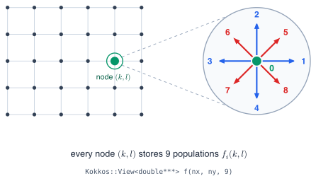
The streaming step moves each population by one lattice site along its direction vector \(\mathbf{c}_i\). At the edge of a rank’s patch, this means some populations leave the patch: after streaming, they belong to a node owned by the neighboring rank. Conversely, the boundary nodes of the patch are missing the populations that should have streamed in from the neighbor. The ghost layer is exactly the place where these incoming populations are received: the neighbor’s outgoing boundary populations are communicated into the local ghost cells, and streaming then proceeds as if the neighbor’s nodes were present.

Crucially, not all nine populations need to be communicated. Only the channels whose direction vector points across a boundary carry information to the other side. For a right boundary these are the channels with \(c_{i,x} = +1\), i.e. \(f_1\), \(f_5\) and \(f_8\); for a left boundary \(f_3\), \(f_6\) and \(f_7\); for a top boundary \(f_2\), \(f_5\) and \(f_6\); and for a bottom boundary \(f_4\), \(f_7\) and \(f_8\). (See the lattice Boltzmann lecture for the D2Q9 definition and the channel table in the boundary conditions lecture – the same channels that interact with a physical wall are the ones that cross a processor boundary.) Figure 6 illustrates this for a 2D decomposition into four tiles.

Figure 6: A 2D lattice Boltzmann domain decomposed into four rank tiles, each surrounded by a one-cell ghost layer (dashed). Only the populations pointing across a boundary must be communicated: \(f_1\), \(f_5\) and \(f_8\) cross the right edge, \(f_2\), \(f_5\) and \(f_6\) the top edge. The diagonal populations \(f_5\)–\(f_8\) land in the corner cells of the diagonal neighbor.

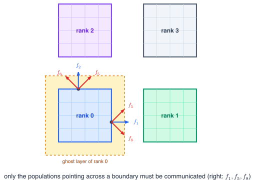
Sending only the crossing channels reduces the communicated volume from nine to three populations per boundary node. Sending all nine is also correct – the extra values are simply ignored – and is a perfectly reasonable first implementation; you can optimize the message size once the code works.

Corners: two sweeps instead of eight neighbors

Figure 6 reveals a complication of 2D decompositions: the diagonal populations \(f_5\)–\(f_8\) stream across the corners of a patch, into the patch of the diagonal neighbor. Does every rank now need eight neighbors and eight messages?

No. The standard trick is to perform the halo exchange in two sweeps, one per axis, and to include the ghost cells of the first sweep in the messages of the second (Figure 7). Sweep 1 exchanges the boundary columns in the \(x\)-direction; after it completes, the left and right ghost columns hold valid neighbor data – including the corner values that arrived from the horizontal neighbors. Sweep 2 then exchanges the boundary rows in the \(y\)-direction, sending the full row including the ghost cells at its ends. The corner data thus travels in two hops – first horizontally, then vertically – and arrives at the diagonal neighbor without a single diagonal message.

Figure 7: Two-sweep corner exchange: sweep 1 exchanges halos in the \(x\)-direction; sweep 2 exchanges halos in the \(y\)-direction and includes the ghost columns filled by sweep 1. Corner data reaches the diagonal neighbor in two hops, without diagonal messages.

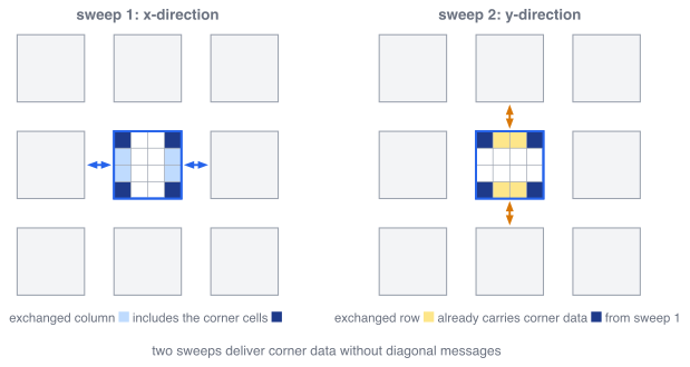
This works for any stencil with a one-cell halo, and it generalizes directly to 3D, where three sweeps over six face-neighbors replace what would otherwise be 26 distinct messages.

Virtual topologies

In 2D, computing neighbor ranks by hand from the rank index is easy to get wrong – especially with periodic wrap-around. MPI can do this bookkeeping for you through a virtual topology: a Cartesian communicator that arranges the ranks in a logical process grid and answers neighbor queries.

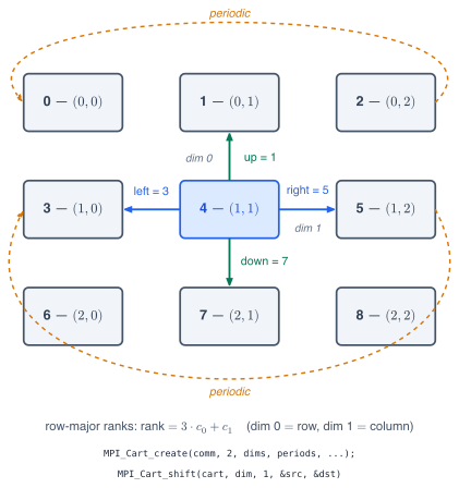
Figure 8: A \(3 \times 3\) periodic Cartesian topology. Each rank is assigned grid coordinates \((c_0, c_1)\); ranks are laid out row-major, \(\text{rank} = 3 c_0 + c_1\). MPI_Cart_shift returns the neighbors of (here) rank 4 along each dimension; the dashed arrows show the periodic wrap-around.

Three functions do all the work. MPI_Dims_create factorizes the number of ranks into a balanced process grid, MPI_Cart_create builds the communicator, and MPI_Cart_shift returns the source and destination rank for a shift along one dimension – exactly the two arguments a halo-exchange MPI_Sendrecv needs:

int size;
MPI_Comm_size(MPI_COMM_WORLD, &size);

// Balanced 2D process grid, e.g. 9 ranks -> dims = {3, 3}
int dims[2] = {0, 0};
MPI_Dims_create(size, 2, dims);

// Periodic Cartesian communicator (periodic in both dimensions)
int periods[2] = {1, 1};
MPI_Comm cart;
MPI_Cart_create(MPI_COMM_WORLD, 2, dims, periods, /* reorder */ 1, &cart);

// Rank and coordinates within the new communicator
int rank, coords[2];
MPI_Comm_rank(cart, &rank);
MPI_Cart_coords(cart, rank, 2, coords);

// The four neighbors; with periodic boundaries every rank has all four
int up, down, left, right;
MPI_Cart_shift(cart, /* dim */ 0, /* displacement */ 1, &up, &down);
MPI_Cart_shift(cart, /* dim */ 1, /* displacement */ 1, &left, &right);

With the row-major layout of Figure 8, rank 4 at coordinates \((1, 1)\) obtains up = 1, down = 7, left = 3 and right = 5. Because the communicator is periodic, the ranks at the edge of the process grid automatically receive their wrapped-around neighbors – no special-casing of the global boundary is needed. (For non-periodic dimensions, MPI_Cart_shift returns MPI_PROC_NULL at the edges, which turns the corresponding MPI_Sendrecv halves into no-ops, just as in the wave solver above.)

Note

With reorder = 1, MPI is allowed to renumber the ranks so that neighboring patches land on physically close hardware. Always query your rank and coordinates from the new communicator, not from MPI_COMM_WORLD.

Strips or tiles?

Should you decompose your 2D domain into 1D strips or 2D tiles? The deciding quantity is the communication volume per rank – the amount of halo data each rank exchanges per time step.

Figure 9: Halo volume per rank for an \(L \times L\) grid on \(p\) ranks: strips exchange two rows of length \(L\) regardless of \(p\), while tiles exchange four edges of length \(L/\sqrt{p}\), which shrinks as \(p\) grows.

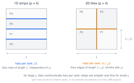
For an \(L \times L\) grid on \(p\) ranks:

• Strips have two boundaries of length \(L\) each, so the halo volume per rank is \(2L\) – independent of \(p\). Adding more ranks shrinks the compute per rank but not the communication per rank, so communication eventually dominates.
• Tiles (a \(\sqrt{p} \times \sqrt{p}\) process grid) have four boundaries of length \(L/\sqrt{p}\), so the halo volume per rank is \(4L/\sqrt{p}\) – it decreases as you add ranks.

Setting \(4L/\sqrt{p} < 2L\) gives the crossover: tiles communicate less per rank once \(p > 4\). Asymptotically the tile decomposition is clearly superior, and for large rank counts it is the only one that scales.

Strips, however, are much simpler: two neighbors, no corner exchange, no process grid. For the modest rank counts of this course, the strip decomposition’s larger halo volume is rarely the bottleneck. The pragmatic recommendation is therefore: start with strips, and generalize to tiles only if your scaling measurements demand it. If you structure your halo exchange as the two sweeps of Figure 7 from the start, the generalization is mostly a matter of using MPI_Dims_create with a \(1 \times p\) grid first and a balanced grid later.

Validation and pitfalls

The decomposed solver must produce the same physics as the serial one. The decisive test – and a requirement of milestone 6 – is to run the identical problem serially and with several rank counts and compare the results: they must agree to numerical precision, since domain decomposition changes only where numbers are computed, not which numbers are computed.

Common pitfalls to check when they do not agree:

• Missing Kokkos::fence() before MPI. GPU kernels run asynchronously; posting an MPI send from device data before the kernel that writes it has finished transmits garbage. See the MPI lecture for the synchronization pattern.
• Off-by-one errors in ghost indexing. Keep the convention explicit and use it everywhere: interior indices 1..n_local, ghosts at 0 and n_local + 1. Sending the ghost cell instead of the outermost interior cell (or receiving into an interior cell) is the classic bug.
• Stale corners. If diagonal data does not arrive, verify that your second sweep includes the ghost cells filled by the first sweep (Figure 7).
• Load imbalance when the grid does not divide evenly. If nx % p != 0, distribute the remainder one extra column to the first nx % p ranks rather than giving the entire remainder to the last rank – otherwise everyone waits for the most loaded rank in every step.
• Not measuring. Whether your decomposition scales is an experimental question. Measure strong (and ideally weak) scaling as described in the scaling notes; milestone 6 asks for these plots.

Further reading

• The process topologies chapter of the MPI standard specifies MPI_Cart_create, MPI_Dims_create and MPI_Cart_shift in full detail.
• Running MPI programs – how to launch your decomposed solver on the cluster.
• Krüger et al. (2017) discusses domain decomposition specifically for lattice Boltzmann solvers.

References

Krüger, Timm, Halim Kusumaatmaja, Alexandr Kuzmin, Orest Shardt, Goncalo Silva, and Erlend Magnus Viggen. 2017. The Lattice Boltzmann Method: Principles and Practice. Springer International Publishing.