Lattice Boltzmann I
From molecules to the lattice
Learning objectives
- Explain how the distribution function \(f(\mathbf{r}, \mathbf{v}, t)\) replaces individual molecules
- Interpret the BGK-Boltzmann equation: streaming vs. collision
- Discretize velocity space with D2Q9 and state the collide-stream algorithm
- Argue why this algorithm is a perfect fit for GPUs (milestones 2 and 3)
A fluid is molecules
- Molecule \(i\): position \(\mathbf{r}_i\), velocity \(\mathbf{v}_i\) – molecular dynamics integrates all of them
- Typical molecular spacing: \(\sim 1\) Å
- A single droplet contains \(\sim 6 \cdot 10^{23}\) molecules
- For anything \(\sim\) meters we need statistics
The distribution function
\[f(\mathbf{r}, \mathbf{v}, t)\]
Probability density of finding a molecule with velocity \(\mathbf{v}\) at position \(\mathbf{r}\) at time \(t\).
- Coarse-grain: average over small cells in position and velocity space
- One function instead of \(6 \cdot 10^{23}\) trajectories
- All of hydrodynamics is encoded in its moments
Moments of \(f\) are the macroscopic fields
\[\rho = m \int \mathrm{d}^D v\, f\] \[\rho \mathbf{u} = m \int \mathrm{d}^D v\, \mathbf{v}\, f\] \[k_B T \propto \int \mathrm{d}^D v\, (\mathbf{v}-\mathbf{u})^2 f\]
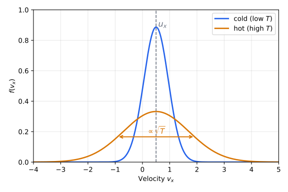
Density = total probability, velocity = its mean, temperature = its spread: hot is broad, cold is narrow.
Equilibrium: the Maxwell distribution
\[
f^\text{eq}(\mathbf{v}; \rho, \mathbf{u}, T) = \frac{\rho}{m}
\left(\frac{m}{2\pi k_B T}\right)^{D/2}
\exp\left\{-\frac{m(\mathbf{v}-\mathbf{u})^2}{2 k_B T}\right\}
\]
A Gaussian centered at the flow velocity \(\mathbf{u}\), with width set by temperature.
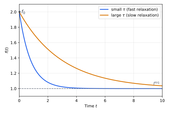
Collisions push \(f\) toward \(f^\text{eq}\)
BGK relaxation-time approximation:
\[\frac{\mathrm{d}f}{\mathrm{d}t} = -\frac{f - f^\text{eq}}{\tau}\]
- One single relaxation time \(\tau\)
- Constant temperature assumed
The Boltzmann transport equation
Chain rule on the total derivative \(\mathrm{d}f/\mathrm{d}t\):
\[
\frac{\partial f}{\partial t}
+ \mathbf{v} \cdot \nabla_{\mathbf{r}} f
+ \frac{\mathbf{F}}{m} \cdot \nabla_{\mathbf{v}} f
= -\frac{f - f^\text{eq}}{\tau}
\]
Left: streaming of probability through phase space. Right: collisions relaxing toward equilibrium.
- For this course we set \(\mathbf{F} = 0\)
Streaming is exact
\[
f(\mathbf{r} + \mathbf{v}\Delta t,\, \mathbf{v},\, t + \Delta t) = f(\mathbf{r}, \mathbf{v}, t)
\]
A packet of probability density simply moves at its own velocity – no approximation involved.
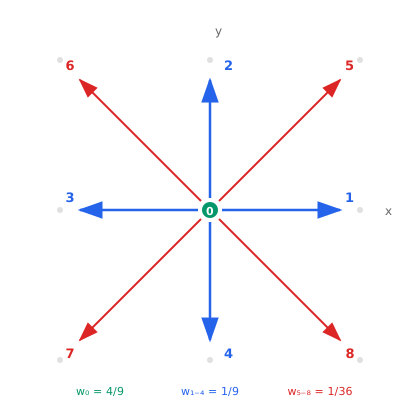
Discretize velocity space: D2Q9
| 0 |
\((0,0)\) |
\(4/9\) |
| 1–4 |
\((1,0), (0,1), (-1,0), (0,-1)\) |
\(1/9\) |
| 5–8 |
\((1,1), (-1,1), (-1,-1), (1,-1)\) |
\(1/36\) |
With \(\Delta t = 1\), every \(\mathbf{c}_i \Delta t\) lands exactly on a neighbor node – streaming stays exact.
The basic data structure: \(f_i(\mathbf{x}, t)\)
- 9 populations \(f_0, \ldots, f_8\) at every lattice site
- On a 2D lattice:
Kokkos::View<double***> f("f", 9, nx, ny)
- Moments become sums: \(\rho = \sum_i f_i\), \(\quad \rho\mathbf{u} = \sum_i \mathbf{c}_i f_i\)
- This array is what you stream in milestone 2
Discrete equilibrium distribution
\[
f_i^\text{eq} = w_i \rho \left[1 + 3\, \mathbf{c}_i \cdot \mathbf{u}
+ \frac{9}{2} (\mathbf{c}_i \cdot \mathbf{u})^2
- \frac{3}{2} u^2\right]
\]
The low-Mach expansion of the Maxwell distribution on the nine velocities; valid for \(|\mathbf{u}| \ll c_s\).
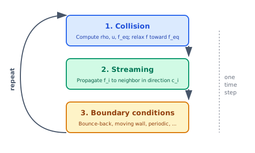
The collide-stream algorithm
![]()
- Collide (local): \(f_i^* = f_i - \omega (f_i - f_i^\text{eq})\), with \(\omega = \Delta t/\tau\)
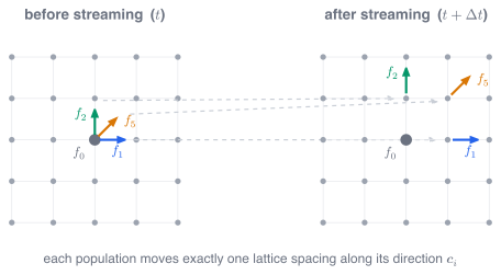
- Stream: \(f_i(\mathbf{x} + \mathbf{c}_i, t+1) = f_i^*(\mathbf{x}, t)\)
- Boundary conditions: next lecture
What streaming does on the lattice
![]()
Every population hops to the neighbor its velocity points to – pure data movement.
Why LBM loves GPUs
- Collision is purely local – every site independent
- Streaming is nearest-neighbor – regular, predictable memory access
- One thread per lattice site, tens of thousands of sites
- Exactly the workload of milestones 2 and 3:
parallel_for over the lattice
Viscosity and stability
Chapman-Enskog analysis connects the LBE to Navier-Stokes:
\[\nu = \frac{1}{3}\left(\frac{1}{\omega} - \frac{1}{2}\right)\]
- Stability window: \(0 < \omega < 2\)
- \(\omega \to 0\): \(\nu \to \infty\) (no relaxation); \(\omega = 1\): full relaxation in one step; \(\omega \to 2\): \(\nu \to 0\), unstable
Summary
- Statistics replaces \(6 \cdot 10^{23}\) molecules: \(f(\mathbf{r}, \mathbf{v}, t)\); moments give \(\rho\), \(\mathbf{u}\), \(T\)
- BGK: collisions relax \(f\) to the Maxwell equilibrium with one time scale \(\tau\)
- D2Q9: nine populations per site; streaming hits neighbor nodes exactly
- Collide (local) + stream (nearest-neighbor) = an algorithm made for GPUs
- \(\omega\) sets the viscosity: \(\nu = \frac{1}{3}(1/\omega - 1/2)\)