Milestone 02
Streaming operator
Learning goals
The student will…
- …understand the streaming step of the Lattice Boltzmann method.
- …set up data structures in their C++ code.
Introduction
The Boltzmann transport equation (BTE) was given in the lecture: \[ \frac{\partial f(\mathbf{r},\mathbf{v},t)}{\partial t}+\mathbf{v}\nabla_{\mathbf{r}} f(\mathbf{r},\mathbf{v},t) +\mathbf{a}\nabla_{\mathbf{v}} f(\mathbf{r},\mathbf{v},t)=C(f(\mathbf{r},\mathbf{v},t)). \tag{1}\] The l.h.s. of this equation is called the streaming term while the r.h.s. is the collision term \(C(f)\). The unknown quantity of Equation 1 is the probability density function \(f(\mathbf{r},\mathbf{v},t)\) which is sometimes also referred to as the distribution function. Unlike other variables, such as for example the density \(\rho(\mathbf{r},t)\) which is just a function of the physical space \(\mathbf{r}\) and the time \(t\), the probability density function \(f(\mathbf{r},\mathbf{v},t)\) presents a dependence also on the velocity \(\mathbf{v}\). This means that we need to discretize \(f\) in space \(\mathbf{r}\), velocity \(\mathbf{v}\) and time \(t\).
- The spatial discretization of \(f\) can be described by a \(n\)-dimensional structured mesh (Figure 1 represents the 2D case) whose grid elements are equidistant.
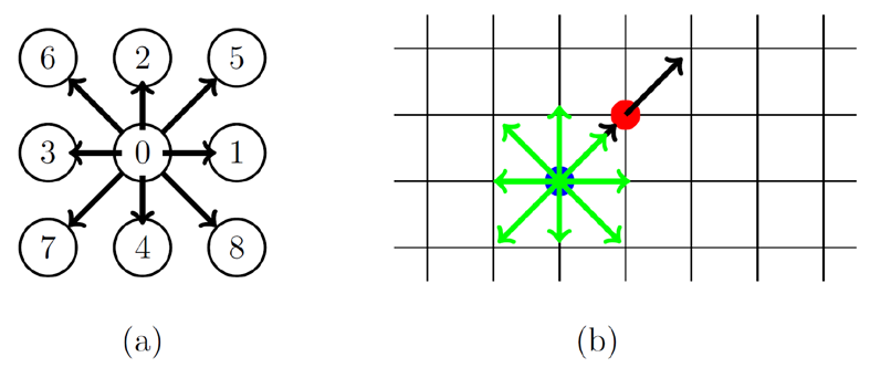
- The velocity space can be discretized by forcing the particle to move along prescribed directions \(\mathbf{c}_i\) which are called “velocity sets”. Figure 1 (a) shows the typical velocity discretization for a 2D case where 9 possible directions are considered. This means that we can substitute the notation \(f(\mathbf{r},\mathbf{v},t)\) though \(f_i(\mathbf{r},t)\), where the index \(i\) refers to the directions shown in Figure 1 (a).
- The time is discretized in time steps \(\Delta t\) during which the values of \(f_i\) are propagated along the corresponding velocity direction \(\mathbf{c}_i\).
The velocity sets \(\mathbf{c}_i\) and the discretization \(\Delta x\) and \(\Delta t\) are chosen so that \(\mathbf{c}_i \Delta t\) points from the current node \(\mathbf{r}\) to the neighbouring ones \(\mathbf{r}+\mathbf{c}_i \Delta t\). This condition is fulfilled if we choose unity values for \(\Delta x\) and \(\Delta t\) and the following velocity set: \[\begin{equation} \mathbf{c} = \left( \begin{array}{ccccccccc} 0 & 1 & 0 & -1 & 0 & 1 & -1 & -1 & 1 \\ 0 & 0 & 1 & 0 & -1 & 1 & 1 & -1 & -1 \end{array}\right)^T. \end{equation}\] In this way the velocity sets (velocity discretization) in Figure 1 can be superimposed to the lattice grid (spatial discretization) in Figure 1.
Thanks to this discretization we can rewrite equation Equation 1 in its discretized form, also known as the lattice Boltzmann equation:
\[\begin{equation} f_i(\mathbf{r}+\mathbf{c}_i\Delta t,t+ \Delta t) = f_i(\mathbf{r}, t) + C_i(\mathbf{r}, t). \end{equation}\]
The value of the discretized probability density function \(f_i\) will move with velocity \(\mathbf{c}_i\) to an adjacent point \(\mathbf{r}+\mathbf{c}_i\Delta t\) at the next time step \(t+ \Delta t\) as shown, for example, with the red particle in Figure 1 (b).
Streaming operator
As first approximation for this milestone, we can focus on the streaming part of the above equation by setting the collision term to zero. In this way we get a transport equation which represents the movement of particles in the vacuum, where no mutual interaction between particles is considered. \[\begin{equation}
f_i(\mathbf{r}+\mathbf{c}_i\Delta t,t+ \Delta t) = f_i(\mathbf{r}, t).
\end{equation}\] In such a scenario, each particle will continue to travel in the vacuum according to Newton’s second law, since the forcing term is zero. Figure 2 shows what your streaming function must do: each population hops one lattice site along its direction per time step.

As further simplification for this milestone we consider periodic boundary conditions, so that the particles which flow outside the domain will re-enter again from the other side.
In summary, the following approximations are made in this milestone:
- Low-density limit (no interaction between particles): collision operator is set to zero (\(C(f)=0\)).
- We will restrict the simulation to a two dimensional space. Velocity is limited to 9 degrees of freedom.
- Periodic boundary condition.
Roadmap
We discretize a 2D domain so that the position vector \(\mathbf{r}\) can be expressed through the two coordinates \(x\) and \(y\).
- The first step is to identify a proper data structure to store the density \(\rho(x,y)\), velocity \(\mathbf{v}(x,y)\) and the distribution function \(f(x,y,\textbf{v})\). Use Kokkos
Viewas your core data structure for such multi-dimensional arrays. Note that the velocity is already discretized into 9 directions by the D2Q9 scheme, so \(f\) can be stored as a three-dimensional array indexed by \((x, y, i)\) where \(i\) is the direction index. - The density is the zeroth moment of the distribution function, \(\rho(x,y) = \int d\textbf{v}\, f(x,y,\textbf{v})\). Since the velocity space is discretized into the 9 directions of the D2Q9 set, this integral becomes a sum over the directions, \[ \rho(x,y) = \sum_i f_i(x,y). \tag{2}\] Write a function which will compute the density at each lattice point.
- The velocity field \(\textbf{u}\) is the first moment of the distribution function divided by the density. In discretized form, \[ \textbf{u}(x,y) = \frac{1}{\rho(x,y)}\sum_i \mathbf{c}_i f_i(x,y). \tag{3}\] Write a function which will compute the velocity field at your grid points. (These are the same expressions you will use again in milestone 3.)
- Initialize the probability density function with values of your choice. We suggest you start with a grid that is \(15\) lattice points wide and \(10\) points long.
- Write a function
streamingwhich shifts the components of the probability density function along the grid according to their direction. Use Kokkosparallel_forto implement this. - You will also need some function to output the fields to a file for later visualization. We suggest you use Python and the library
matplotlibto visualize your results. - Optional: create a short animation that shows how the velocity field travels in time.
Validation
The streaming operator is simple enough that you can verify it exactly:
- Initialize a single non-zero “blob” of populations (a small patch of lattice points with a non-zero value in one direction \(i\), everything else zero) and stream with periodic boundary conditions. The pattern must translate by one lattice site per time step along \(\mathbf{c}_i\) without changing its shape.
- Because the boundary conditions are periodic, the blob must return exactly to its initial position after \(N_x\) steps (for a horizontally moving direction) or \(N_y\) steps (for a vertically moving one). Compare the field after this round trip with the initial condition — the two must be identical.
- The total mass \(\sum_{x,y,i} f_i(x,y)\) must be conserved to machine precision at every time step, since streaming only moves values around. Add a check (and a unit test) for this invariant.
Suggestions
- The probability density function \(f(\mathbf{r}, \mathbf{v},t)\) has a non trivial physical meaning. Therefore we suggest, at the beginning, to think of the value of \(f_i(\mathbf{r},t)\) as the number of “particles” which are in the position \(\mathbf{r}\) at the time \(t\) and that are moving in the direction \(\mathbf{c_i}\).
- Test the streaming function by initialising \(f_i\) in a simple way with values only in few (or even one) direction.
- In order to visualize your velocity field, we would suggest the use of the streamplot function in matplotlib.pyplot. However this approach is mainly suggested for the coming milestones where the velocity field has a proper physical meaning.