Scientific and parallel computing
A brief history of scientific computing
This class deals with scientific computing on high-performance computing (HPC) systems, sometimes also termed supercomputers. These are massively parallel machines that require parallel programming approaches for their use.
After working through this lecture, you should be able to:
- outline the historical development from vector machines to massively parallel, GPU-accelerated supercomputers,
- describe the tiered HPC ecosystem in Germany and Europe and the levels of hardware parallelism in a modern cluster,
- define speedup and parallel efficiency, and distinguish strong from weak scaling,
- apply Amdahl’s and Gustafson’s laws and explain which question each of them answers.
Scientific computing – the use of computers to solve scientific and engineering problems numerically – has a rich history that is inseparable from the development of computers themselves.
The early days: Los Alamos and the birth of computing
The first general-purpose electronic computers were built to solve scientific problems. ENIAC (1945) at the University of Pennsylvania was used for ballistics calculations and early hydrogen bomb simulations. Shortly after, the MANIAC (Mathematical Analyzer Numerical Integrator and Computer, 1952) at Los Alamos National Laboratory was built specifically for nuclear weapons research. It was on MANIAC that some of the earliest computational physics simulations were carried out, including the Metropolis Monte Carlo method (Metropolis, Rosenbluth, Rosenbluth, Teller & Teller, 1953), which introduced stochastic sampling for computing equations of state, and the celebrated Fermi–Pasta–Ulam–Tsingou numerical experiment (1955), which revealed unexpected recurrence in nonlinear dynamical systems and launched the field of computational nonlinear science. The pioneering molecular dynamics work by Alder and Wainwright followed in the late 1950s on an IBM 704 at Livermore.
Throughout the 1960s and 1970s, scientific computing drove computer architecture. Seymour Cray designed a series of increasingly powerful machines – the CDC 6600 (1964, the first supercomputer), the CDC 7600, and the Cray-1 (1976) – that introduced vector processing, allowing a single instruction to operate on multiple data elements simultaneously. Vector machines dominated scientific computing through the 1980s.
The parallel era
The 1990s brought a paradigm shift: instead of building ever-faster single processors, supercomputers were assembled from large numbers of commodity processors connected by high-speed networks. This massively parallel approach required new programming models, most notably the Message Passing Interface (MPI), standardized in 1994, which remains the dominant distributed-memory programming model today.
The 2000s saw the rise of multi-core CPUs, where parallelism moved inside each processor chip. Single-threaded performance improvements, which had doubled roughly every two years following Moore’s law, slowed dramatically around 2005 as power consumption and heat dissipation hit physical limits (the “power wall”). Further performance gains now come almost exclusively from parallelism.
The accelerator era
Since the 2010s, GPUs and other accelerators have become a dominant force in high-performance computing. Originally designed for graphics rendering, GPUs were found to excel at the regular, data-parallel computations common in scientific simulations. Today, the majority of floating-point performance in the world’s fastest supercomputers comes from GPU accelerators. The TOP500 list of the world’s most powerful supercomputers is led by GPU-accelerated systems.
This shift has created a challenge: each GPU vendor (NVIDIA, AMD, Intel) promotes its own programming model (CUDA, HIP/ROCm, SYCL). Hardware abstraction layers such as Kokkos have emerged to provide portable code that runs efficiently across different accelerator architectures. Kokkos is the hardware abstraction layer used in this class.
The HPC ecosystem in Germany and Europe
High-performance computing resources are organized in a tiered hierarchy, both within Germany and at the European level. The tiers reflect increasing computational power and decreasing accessibility:
German tier system
The Gauß-Allianz coordinates the German HPC ecosystem, which is organized into four tiers:
| Tier | Scale | Access | Examples |
|---|---|---|---|
| Tier 3 | State-level entry clusters, departmental clusters | Researchers at state universities; registration required | bwUniCluster (KIT), bwForCluster NEMO (Freiburg) |
| Tier 2 | National mid-range supercomputers (NHR centers) | Researchers nationwide; application with scientific justification | HoreKa (KIT, >60k cores, >750 NVIDIA GPUs), Helma (FAU Erlangen), Lichtenberg II (TU Darmstadt) |
| Tier 1 | National flagship supercomputers | Peer-reviewed proposal required | JUPITER (JSC Jülich, €500M1), SuperMUC-NG (LRZ Munich), Hunter (HLRS Stuttgart, €200M1) |
| Tier 0 | European flagship systems | International peer review via EuroHPC | LUMI (Finland, €200M1), Leonardo (Italy, €240M2), MareNostrum 5 (Spain) |
1Total cost of ownership (hardware, power, cooling, operations). 2Hardware acquisition cost.
The three Tier 1 centers – JSC (Jülich), LRZ (Munich) and HLRS (Stuttgart) – form the Gauss Centre for Supercomputing (GCS). Through GCS, the German Tier 1 systems also serve as European Tier 0 resources within the EuroHPC infrastructure, in particular JUPITER which is co-funded by EuroHPC JU. The National High-Performance Computing alliance (NHR) coordinates the Tier 2 centers, currently nine NHR centers at German universities.
In Baden-Württemberg, the state-funded bwHPC program operates the Tier 3 systems. The bwUniCluster at KIT is a general-purpose cluster available to all universities in the state (393 nodes, ~28k cores, 188 GPUs). The bwForCluster NEMO in Freiburg serves specific research communities including microsystems engineering and materials science. The Tier 2 system at KIT is HoreKa, a hybrid supercomputer with over 60,000 processor cores and more than 750 NVIDIA GPUs (A100, H100, H200).
European HPC: EuroHPC
The EuroHPC Joint Undertaking is an EU initiative that funds and operates Tier 0 (pre-exascale and exascale) systems across Europe. The first European exascale system JUPITER at Forschungszentrum Jülich in Germany is based on NVIDIA Grace-Hopper superchips. LUMI in Finland (AMD MI250X GPUs) and Leonardo in Italy (NVIDIA A100 GPUs) are the largest operational EuroHPC systems.
Practical relevance for this class
In this class, you will primarily use:
- Tier 3: the bwUniCluster at KIT for development, testing and parallel scaling experiments.
Hardware architectures
Parallel hardware has become ubiquitous. Most central processing units (CPUs) in computers, phones or other hardware have multiple cores that can execute instructions in parallel. Massively parallel computing systems combine multiple CPUs into nodes that share a common memory. These nodes are then combined into the full compute system through a network interconnect.
Parallel architectures are often hierarchical and have parallelization at different levels:
- Vectorization (SIMD) at the core level: a single instruction operates on multiple data elements. Modern CPUs have vector units that can process 4–16 double-precision floating-point numbers per cycle (SSE, AVX2, AVX-512).
- Shared-memory parallelization for multicore architectures: multiple cores within a node share the same physical memory and can communicate through that memory. Programming models include threads (pthreads, C++
std::thread) and OpenMP. - Distributed-memory parallelization for large computing systems: nodes communicate via a network interconnect using message passing. The dominant programming model is MPI.
- Accelerator parallelization using GPUs or other devices: massively parallel processors with thousands of simple cores, connected to the CPU via PCIe or NVLink. Programming models include CUDA, HIP, SYCL and hardware abstraction layers like Kokkos.
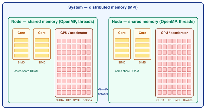
The GPU architecture lecture explains the accelerator level in detail.
Parallel scaling
Software that runs on parallel computers needs to scale. Scaling describes how the time to solution changes as the number of available compute units (cores or processes) increases.
Speedup and efficiency
The most basic metric is the speedup \(S\), defined as the ratio of serial to parallel execution time: \[S(p) = \frac{T_1}{T_p}\] where \(T_1\) is the time to solution on a single process and \(T_p\) is the time on \(p\) processes. Ideal (linear) scaling gives \(S = p\): doubling the number of processes halves the time.
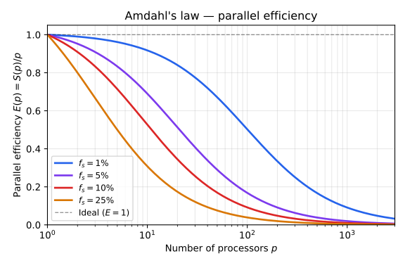
The parallel efficiency measures how well the available resources are utilized. For a fixed problem size (strong scaling, see below) it is defined as \[E_s(p) = \frac{S(p)}{p} = \frac{T_1}{p \, T_p}\] An efficiency of \(E_s = 1\) (or 100%) means perfect scaling. In practice, efficiency decreases with increasing \(p\) due to communication overhead, load imbalance, and serial bottlenecks.
Amdahl’s law
The simplest model for scaling assumes that a program can be divided into a serial fraction \(f_s\) and a parallel fraction \(f_p = 1 - f_s\). On a single process, the total execution time is \(T_1\), of which \(f_s T_1\) is spent in the serial part and \(f_p T_1\) in the parallel part. On \(p\) processes, only the parallel part is divided: \[T_p = f_s T_1 + \frac{f_p T_1}{p}\]
The speedup is therefore: \[S(p) = \frac{T_1}{T_p} = \frac{T_1}{f_s T_1 + f_p T_1 / p} = \frac{1}{f_s + f_p / p} = \frac{p}{f_s p + f_p}\]
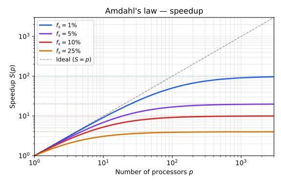
This is Amdahl’s law. In the limit of infinitely many processors (\(p \to \infty\)), the speedup saturates at: \[S_\text{max} = \frac{1}{f_s}\]
The following table illustrates how even a small serial fraction severely limits scalability:
| \(f_s\) | \(S(p{=}10)\) | \(S(p{=}100)\) | \(S(p{=}1000)\) | \(S_\text{max}\) |
|---|---|---|---|---|
| 1% | 9.2 | 50.3 | 91.0 | 100 |
| 5% | 6.9 | 16.8 | 19.6 | 20 |
| 10% | 5.3 | 9.2 | 9.9 | 10 |
| 25% | 3.1 | 3.9 | 4.0 | 4 |
With \(f_s = 5\%\), going from 100 to 1000 processes barely improves the speedup (16.8 to 19.6). The serial fraction is the bottleneck.
Strong and weak scaling
Amdahl’s law describes strong scaling: the problem size is fixed and we increase the number of processes to reduce the time to solution. Strong scaling is the relevant metric when you have a specific simulation to run and want to know how much faster it gets with more resources. Figure 3 shows how quickly the strong-scaling efficiency \(E_s(p)\) deteriorates under Amdahl’s law: even with a serial fraction of only 1%, efficiency drops to about 50% at \(p = 100\).
However, in scientific computing we often want to solve larger problems, not just solve the same problem faster. Weak scaling keeps the workload per process fixed and increases the number of processes to tackle a proportionally larger problem. The metric is the weak-scaling efficiency \(E_w(p) = T_1 / T_p\), which ideally remains at 100% (flat line) as \(p\) grows. Note that the two efficiency definitions differ deliberately: in strong scaling the same total work is shared by \(p\) processes, so ideal scaling means \(T_p = T_1/p\) and we must divide by \(p\); in weak scaling \(T_p\) is measured on a \(p\)-times larger problem, so ideal scaling simply means \(T_p = T_1\).
Gustafson’s law
Amdahl’s law is pessimistic because it assumes a fixed problem size. In practice, the serial fraction often decreases as the problem grows. Consider a simulation on an \(N \times N\) grid: the computation scales as \(O(N^2)\) but the serial overhead (initialization, I/O, global reductions) may scale as \(O(N)\) or \(O(1)\). As \(N\) increases, the serial fraction \(f_s\) shrinks.
Gustafson’s law formalizes this by assuming fixed parallel execution time rather than fixed problem size. If we define \(f_s'\) as the serial fraction measured on the parallel run (i.e. on \(p\) processes), the scaled speedup is: \[S(p) = f_s' + p \, (1 - f_s') = p - f_s'(p - 1)\]
This gives a speedup that grows linearly with \(p\), reduced only by the serial overhead \(f_s'\). Gustafson’s law explains why large-scale simulations can scale efficiently to thousands of processes even when Amdahl’s law would predict saturation: the problem is scaled up together with the number of processes.
Worked example. Take a serial fraction of 5% and \(p = 100\) processes. Amdahl’s law (fixed problem size) gives \[S = \frac{1}{0.05 + 0.95/100} \approx 16.8,\] while Gustafson’s law (problem size grown with \(p\)) gives \[S = 100 - 0.05 \times 99 = 95.05.\] The two results are not contradictory – they answer different questions. Amdahl asks: how much faster can I solve this fixed problem? (Answer: at most 20x, no matter how many processes.) Gustafson asks: how much more work can I do in the same wall-clock time? (Answer: nearly 100x.) Which law is relevant depends on whether you want to shorten the time to solution or to enlarge the problem.
Practical considerations
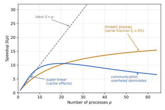
Real parallel codes deviate from both laws due to:
- Communication overhead: exchanging data between processes takes time that grows with \(p\) (more neighbors, more messages). This overhead is not captured by the serial fraction \(f_s\).
- Load imbalance: if the work is not evenly distributed, some processes idle while others compute. This reduces efficiency.
- Memory effects: as the local problem per process shrinks (strong scaling), it may fit entirely in cache, leading to super-linear speedup (\(S > p\)) – a welcome anomaly.
Figure 4 combines these effects into the strong-scaling curve you will typically measure in practice.
The notes on parallel scaling provide practical guidance and examples of measuring strong and weak scaling.