Memory Performance: Caching and Coalescence
Overview
Building on the GPU architecture lecture, we now look at how memory access patterns determine real-world performance. Modern CPUs and GPUs are incredibly fast at computation, but memory access is often the bottleneck in real applications. A single floating-point operation might complete in 1-2 nanoseconds, but fetching data from main memory can take hundreds of nanoseconds. This lecture explains why memory layout matters for performance and how CPUs and GPUs handle memory access differently through caching and memory coalescing.
By understanding these concepts, you’ll be able to: - Write code that’s cache-friendly on CPUs - Write code that uses GPU memory efficiently (coalescence) - Understand why the same algorithm can have vastly different performance on different hardware
Why Memory Matters
Let’s start with a concrete example. Consider this simple loop:
// Bad: random memory access
for (int i = 0; i < 1000000; i++) {
  int idx = rand() % N;  // Random index
  sum += data[idx];
}

// Good: sequential memory access
for (int i = 0; i < N; i++) {
  sum += data[i];
}
Both loops do the same computation (sum all elements), but the second one is typically 10-100x faster because of how memory access is organized. This difference comes from caching and memory hierarchies.
Memory Hierarchy
Modern computers have multiple levels of memory, each with different sizes and speeds:
                    Tiny (Bytes)     Very Fast (1-2 ns)    CPU Registers
                         ↓
                  Small (KBs)        Fast (3-5 ns)        L1 Cache
                         ↓
                 Medium (100s KB)    Medium (12-20 ns)    L2 Cache
                         ↓
              Large (MBs)           Slower (40-75 ns)     L3 Cache (Shared)
                         ↓
        Very Large (100s of GB)   Slow (100-300 ns)      Main Memory (RAM)
                         ↓
        Enormous (TBs)            Very Slow (ms)         Storage (Disk/SSD)
On CPUs, caching happens automatically. The hardware detects memory access patterns and keeps frequently accessed data in fast caches. But this automatic caching is limited—if you access data in a random pattern, the caches can’t help.
CPU Cache: Understanding Cache Lines
CPUs fetch memory in small chunks called cache lines (typically 64 bytes). When you access a single byte, the CPU fetches the entire cache line into the cache (Figure 1).
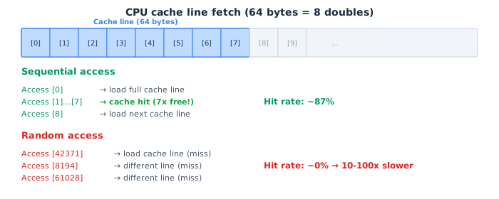
Here’s what happens:
Memory Layout:  [data[0]][data[1]][data[2]][data[3]]...[data[7]]...
                 ↑──────────── One cache line (64 bytes) ──────────↑
If you access data[0], you automatically get data[0] through data[7] (for 8-byte doubles) in the cache.
Sequential access (cache-friendly)
for (int i = 0; i < N; i++) {
  sum += data[i];
}
When the processor accesses data[0], it loads the entire 64-byte cache line containing data[0] through data[7] (for 8-byte doubles) into the L1 cache. The subsequent accesses to data[1], data[2], …, data[7] are all served from the cache without touching main memory. Only when the loop advances past the end of the cache line does a new load occur. The result is a cache hit rate of roughly 87% (7 out of 8 accesses per cache line are hits), and the effective memory latency is close to the L1 latency of a few nanoseconds rather than the hundreds of nanoseconds of main memory.
Random access (cache-unfriendly)
for (int i = 0; i < 1000000; i++) {
  int idx = random_index();
  sum += data[idx];
}
When the access pattern is random, each load is likely to target a different cache line. The cache line fetched for data[idx] is evicted before any of its neighbors are used, resulting in a cache miss rate close to 100%. Every access pays the full main memory latency, and the hardware prefetcher – which detects sequential or strided patterns – cannot help. The loop runs 10–100x slower than the sequential version, despite performing exactly the same arithmetic.
CPU Cache Optimization: Multi-Dimensional Arrays
For multi-dimensional arrays, the layout in memory determines performance:
Row-Major Layout (C/C++ default)
// C++ array layout in memory (row-major)
// A[0][0], A[0][1], A[0][2], ..., A[1][0], A[1][1], ...

double A[M][N];

// GOOD: Access row-by-row (sequential in memory)
for (int i = 0; i < M; i++) {
  for (int j = 0; j < N; j++) {
    sum += A[i][j];  // Sequential access
  }
}

// BAD: Access column-by-column (non-sequential in memory)
for (int j = 0; j < N; j++) {
  for (int i = 0; i < M; i++) {
    sum += A[i][j];  // Jumps around memory
  }
}
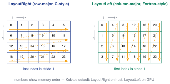
The first version is often 10x faster because accessing row-by-row follows memory layout. The second jumps by N * sizeof(double) bytes each time, missing the cache repeatedly. Figure 2 shows the two possible storage orders and which loop index is contiguous in each.
Actual Performance
On a modern CPU with a matrix of 10,000 × 10,000 doubles (800 MB), one might observe:
- Row-major access: ~2 seconds
- Column-major access: ~20 seconds
- Difference: 10x speedup purely from memory layout
These are illustrative figures; the exact ratio depends on cache sizes, prefetcher behavior and compiler optimizations. Measure on your own hardware – see the benchmarking notes for how to do this reliably.
GPU Memory: Coalescence
GPUs handle memory very differently than CPUs. GPUs do have automatic caches (L1/L2), but they are small relative to the enormous number of concurrent threads, so cache hits cannot be relied upon the way they are on CPUs (see the GPU architecture lecture). Instead, GPUs rely primarily on memory coalescing.
What is Memory Coalescence?
When multiple GPU threads access memory simultaneously, the GPU groups these accesses together into a single transaction. This is efficient when: 1. Threads access consecutive memory addresses 2. The memory access pattern is predictable
Think of it like a bank teller: serving customers one-by-one is slow, but if multiple customers line up in order (addresses 0, 1, 2, … in sequence), the teller can process them all in one batch efficiently (coalesced access).
Coalesced access (GPU-friendly)
// GPU kernel - all threads access consecutive memory
Kokkos::parallel_for(N, KOKKOS_LAMBDA(int i) {
  result[i] = data[i] * 2.0;  // Thread i accesses data[i]
});
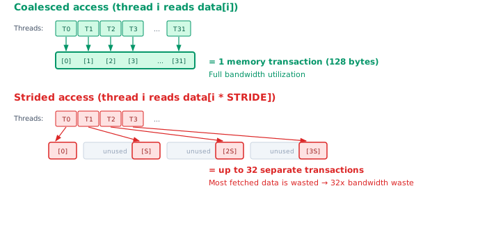
All 32 threads in a warp execute the load instruction simultaneously. Thread 0 requests data[0], thread 1 requests data[1], and so on up to thread 31 requesting data[31]. Because these 32 addresses are contiguous, the GPU’s memory controller combines them into a single 128-byte memory transaction. The result is that 32 loads are served at the cost of one: the memory bus is used at full efficiency.
Non-coalesced access (GPU-unfriendly)
// AVOID: Threads access scattered memory
Kokkos::parallel_for(N, KOKKOS_LAMBDA(int i) {
  int idx = (i * STRIDE) % N;  // Large stride causes poor coalescence
  result[i] = data[idx] * 2.0;
});
With a large stride, thread 0 requests data[0], thread 1 requests data[STRIDE], thread 2 requests data[2*STRIDE], and so on. These addresses fall into different 128-byte segments of memory, and each segment requires a separate memory transaction. In the worst case, 32 threads generate 32 independent transactions – using 32x more bandwidth than the coalesced case for the same amount of useful data. The memory bus is saturated transporting data that is mostly discarded.
Memory Layout for GPUs
Similar to CPUs, memory layout matters on GPUs:
Good (contiguous data):
Kokkos::View<double*> data("data", N);  // Contiguous memory
double sum = 0.0;
Kokkos::parallel_reduce(N, KOKKOS_LAMBDA(int i, double& local_sum) {
  local_sum += data[i];  // Coalesced access
}, sum);
Bad (scattered data):
std::vector<double*> pointers;  // Array of pointers to scattered memory
double sum = 0.0;
Kokkos::parallel_reduce(N, KOKKOS_LAMBDA(int i, double& local_sum) {
  local_sum += *pointers[i];  // Indirect access, hard to coalesce
}, sum);
Note that summing values is a reduction and therefore uses Kokkos::parallel_reduce with a thread-private accumulator (see the Kokkos lecture); accumulating into a shared variable from a parallel_for would be a data race.
CPU vs. GPU Memory Requirements
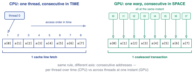
The two architectures reward the same underlying principle – contiguous access – through different mechanisms, as Figure 4 shows side by side. Here’s a summary of how CPUs and GPUs differ:
| Aspect | CPU | GPU |
|---|---|---|
| Memory Access Latency | High (100-300 ns) | Very High (400-1000 ns) |
| Cache Strategy | Automatic caching (large caches) | Coalescing (smaller automatic caches) |
| Optimal Pattern | Sequential or temporal locality | Coalesced (all threads access nearby addresses) |
| Array Layout | Row-major: Access rows sequentially | Coalesced: Threads map to contiguous memory |
| Stride Tolerance | Can handle large strides (cache takes care of it) | Stride of 1 is best; larger strides kill performance |
| Bandwidth | Moderate (50-200 GB/s) | Very High (500+ GB/s) when coalesced |
Compute-bound vs. memory-bound operations
Understanding memory access patterns is important because most scientific codes are not limited by the processor’s arithmetic throughput – they are limited by how fast data can be moved to and from memory. This section introduces the quantitative framework for distinguishing the two regimes.
Arithmetic intensity
The key quantity is the arithmetic intensity \(I\), defined as the number of floating-point operations (flops) performed per byte of data transferred between memory and the processor:
\[I = \frac{\text{flops}}{\text{bytes transferred}}\]
A kernel that performs many operations on each loaded value has high arithmetic intensity. A kernel that loads data, does little work, and moves on has low arithmetic intensity.
Two performance regimes
Every processor has two hardware limits:
- Peak compute performance \(\pi\) (in flop/s): the maximum rate at which arithmetic operations can be executed.
- Peak memory bandwidth \(\beta\) (in byte/s): the maximum rate at which data can be streamed from memory.
For a kernel with arithmetic intensity \(I\), the achievable performance \(P\) (in flop/s) is bounded by both limits:
\[P \leq \min(\pi,\; I \cdot \beta)\]
This gives two regimes:
- Memory-bound (\(I < \pi / \beta\)): the processor finishes its arithmetic before the next data arrives. Performance is limited by bandwidth: \(P \approx I \cdot \beta\). Making the arithmetic faster (e.g. using FMA instructions) does not help – the processor is waiting for data.
- Compute-bound (\(I > \pi / \beta\)): the data arrives before the processor finishes its arithmetic. Performance is limited by peak flop/s: \(P \approx \pi\). Optimizing memory access patterns does not help – the processor is busy computing.
The crossover point \(I^* = \pi / \beta\) is called the machine balance or ridge point. For an NVIDIA A100 GPU (\(\pi \approx 9.7\) Tflop/s FP64, \(\beta \approx 2.0\) TB/s), the ridge point is:
\[I^* = \frac{9.7 \times 10^{12}}{2.0 \times 10^{12}} \approx 4.9 \;\text{flop/byte}\]
Any kernel with \(I < 4.9\) flop/byte is memory-bound on the A100. As we will see, this includes most scientific computing kernels.
The roofline model
The relationship above can be visualized as the roofline model, a log-log plot of achievable performance versus arithmetic intensity (Figure 5).
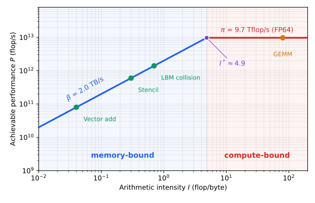
The “roofline” consists of two segments: a sloped line \(P = I \cdot \beta\) on the left (memory-bound region) and a flat ceiling \(P = \pi\) on the right (compute-bound region). A kernel’s arithmetic intensity determines where it falls on the horizontal axis and thus which roof it hits.
Most scientific codes are memory-bound
Consider some common operations and their arithmetic intensities:
| Operation | Flops per element | Bytes per element | \(I\) (flop/byte) |
|---|---|---|---|
| Vector addition \(c_i = a_i + b_i\) | 1 | 24 (read \(a\), \(b\); write \(c\)) | 0.04 |
| Scalar multiply \(b_i = \alpha a_i\) | 1 | 16 (read \(a\); write \(b\)) | 0.06 |
| Dot product \(s = \sum a_i b_i\) | 2 | 16 (read \(a\), \(b\)) | 0.13 |
| 5-point stencil (2D Laplacian) | 5 | 16 (read 5 neighbors; write 1; with caching) | ~0.3 |
| Dense matrix-vector product (\(N{\times}N\)) | \(2N\) | ~\(8N\) (matrix row + vectors) | ~0.25 |
| Dense matrix-matrix product (\(N{\times}N\)) | \(2N^3\) | \(3 \times 8N^2\) | ~\(0.08 N\) |
Vector operations, stencils, and matrix-vector products all have \(I \ll 1\) flop/byte – far below the ridge point of any modern processor. They are deeply memory-bound: performance is determined almost entirely by memory bandwidth, not arithmetic speed.
Only dense matrix-matrix multiplication has an arithmetic intensity that grows with problem size (as \(O(N)\)), which is why it is the one operation that can approach peak flop/s on large matrices. This is the exception, not the rule.
Example: Lattice Boltzmann streaming step
The streaming step of the Lattice Boltzmann method (used throughout this class) moves the 9 population values \(f_i\) at each lattice site to their neighbors. For a D2Q9 lattice:
- Flops per site: essentially 0 (the streaming step only copies data to neighboring sites).
- Bytes per site: \(9 \times 8 = 72\) bytes read + 72 bytes written = 144 bytes.
The arithmetic intensity is \(I \approx 0\) flop/byte – this is a purely memory-bound operation. Its performance is entirely determined by memory bandwidth. On a GPU with 2 TB/s bandwidth, the maximum streaming throughput is roughly \(2 \times 10^{12} / 144 \approx 14 \times 10^9\) lattice site updates per second. No amount of arithmetic optimization can improve this; only memory access patterns (coalescing, layout) matter.
The collision step has a higher arithmetic intensity (computing the equilibrium distribution involves ~100 flops per site against the same 144 bytes), giving \(I \approx 0.7\) flop/byte. This is still well below the ridge point, so the collision step is also memory-bound on current hardware.
Implications for optimization
The fact that most scientific codes are memory-bound has important consequences:
- Memory access patterns matter more than arithmetic tricks. Optimizing for coalesced access (GPU) or cache-friendly access (CPU) – as discussed in the previous sections – delivers larger speedups than reducing the flop count.
- Peak flop/s is a misleading metric. A GPU may advertise 10 Tflop/s, but a memory-bound code will achieve a small fraction of that. The relevant hardware specification is memory bandwidth, not peak compute.
- Data layout choices (LayoutLeft vs LayoutRight, AoS vs SoA) directly impact performance because they determine whether memory transactions are used efficiently.
Practical Example: Matrix Multiplication
Let’s see how memory layout affects a real algorithm:
CPU-Optimized Version
// CPU version: iterate in cache-friendly order
for (int i = 0; i < M; i++) {
  for (int j = 0; j < K; j++) {
    double a_ij = A[i][j];
    for (int k = 0; k < N; k++) {
      C[i][k] += a_ij * B[j][k];  // Accesses C and B sequentially
    }
  }
}
Why is this cache-friendly? - Inner loop accesses B[j][k] and C[i][k] with stride 1 (sequential) - Data from one cache line is reused multiple times - Compiler can prefetch next cache lines
GPU Version
// GPU version: one thread per output element
Kokkos::View<double**> A("A", M, K);
Kokkos::View<double**> B("B", K, N);
Kokkos::View<double**> C("C", M, N);

Kokkos::parallel_for(
  Kokkos::MDRangePolicy<Kokkos::Rank<2>>({0, 0}, {M, N}),
  KOKKOS_LAMBDA(int i, int j) {
    double sum = 0.0;
    for (int k = 0; k < K; k++) {
      sum += A(i, k) * B(k, j);
    }
    C(i, j) = sum;
  });
Why does this work reasonably well on a GPU? - Each thread computes one output element; neighboring threads compute neighboring elements of C - In each iteration of the k-loop, neighboring threads read neighboring elements of B (and the same element of A), so the loads are largely coalesced with the default device layout
Be aware of what this simple version does not do: every thread re-reads its full row of A and column of B from global memory, so there is no data reuse between threads. A genuinely tiled implementation stages blocks of A and B in shared memory using TeamPolicy with team scratch memory (introduced in the Kokkos lecture), which is how optimized libraries approach peak performance. For production code, use a vendor BLAS (cuBLAS, rocBLAS) rather than writing matrix multiplication yourself.
Memory Layout in Kokkos
Kokkos provides different layouts to control memory organization:
Layout Right (Row-Major)
Kokkos::View<double**, Kokkos::LayoutRight> A("A", M, N);
// Memory layout: [A(0,0)][A(0,1)]...[A(0,N-1)][A(1,0)][A(1,1)]...
// Rightmost index is fastest-changing (C/C++ convention)
Layout Left (Column-Major)
Kokkos::View<double**, Kokkos::LayoutLeft> B("B", M, N);
// Memory layout: [B(0,0)][B(1,0)]...[B(M-1,0)][B(0,1)][B(1,1)]...
// Leftmost index is fastest-changing (Fortran convention)
The default layout depends on the memory space
If you do not specify a layout, Kokkos chooses one based on the View’s memory space:
HostSpace(CPU):LayoutRight. A single thread iterating over the rightmost index then walks through memory sequentially, which is cache-friendly.CudaSpace/HIPSpace(GPU):LayoutLeft. Consecutive GPU threads are typically assigned consecutive values of the leftmost index, so withLayoutLeftthey access consecutive memory addresses – exactly the coalesced pattern from Figure 3.
This per-memory-space choice is the reason the same Kokkos kernel can achieve good memory performance on both architectures. Override the default only when interfacing with external libraries (e.g. Fortran or BLAS routines that expect a specific layout) or when profiling shows that your access pattern does not match the default.
// Same kernel, default layout: cache-friendly on the CPU (LayoutRight),
// coalesced on the GPU (LayoutLeft)
Kokkos::View<double**> B("B", M, N);
Kokkos::parallel_for(
  Kokkos::MDRangePolicy<Kokkos::Rank<2>>({0, 0}, {M, N}),
  KOKKOS_LAMBDA(int i, int j) {
    result(i, j) = B(i, j) * 2.0;
  });
Common Pitfalls
Most pitfalls are violations of the access-pattern rules discussed above; we list them here briefly rather than re-explaining them.
Column-wise access on CPU. Iterating over the slow (first) index in the inner loop of a row-major array jumps by
N * sizeof(double)bytes per access and misses the cache repeatedly – see CPU Cache Optimization. Swap the loop order so the fastest-changing index is innermost.Large strides on GPU. An access like
data[i * large_stride]places the addresses of consecutive threads in different memory segments and prevents coalescing (Figure 3). Use unit stride – threadiaccesses elementi– whenever possible.Indirect memory access.
data[indices[i]]with unpredictable indices defeats both CPU caches and GPU coalescing, as discussed in Why Memory Matters. If possible, sort the indices or restructure the data so that accesses become sequential.Accumulating into a shared variable. This one is a correctness bug, not just a performance problem:
// Bad: data race -- all threads write to the same variable
Kokkos::parallel_for(N, KOKKOS_LAMBDA(int i) {
  sum += data[i];
});

// Good: parallel_reduce with a thread-private accumulator
double sum = 0.0;
Kokkos::parallel_reduce(N, KOKKOS_LAMBDA(int i, double& local_sum) {
  local_sum += data[i];
}, sum);
Measuring Memory Performance
CPU: Cache Misses
Use profiling tools to measure cache behavior:
# Linux: Use perf to measure cache misses
perf stat -e cache-references,cache-misses ./program

# Output might show:
# 1,234,567 cache-references (2.15%)
#   123,456 cache-misses   (10.0% of all cache refs)
Lower cache-miss percentage is better. Aim for < 5%.
GPU: Memory Bandwidth
Check if your GPU code is bandwidth-bound:
// Measure time and data transferred
double bandwidth_gb_s = (2 * N * sizeof(double)) / (time_seconds * 1e9);

// Compare to peak bandwidth
// A100: 2 TB/s peak
// RTX 3090: 930 GB/s peak
// If measured << peak, your code is not coalescing well
Guidelines for Writing Performant Code
These guidelines help you write code that performs well on real hardware. For memory-bound kernels, following them can make an order-of-magnitude difference in runtime.
For CPUs
- Access data sequentially when possible - The cache is your friend for sequential patterns
- Iterate over fastest-changing dimension last (for row-major arrays) - This matches how data is stored in memory
- Avoid random memory access - Unpredictable patterns defeat the hardware’s prefetching mechanisms
- Consider blocking/tiling for large arrays - Keep frequently-used data in the fast L1/L2 caches
- Reuse data within inner loops - Each byte of data should be used multiple times after loading
For GPUs
- Ensure coalesced memory access - All threads in a warp should access nearby memory; this is critical for performance
- Use unit stride when possible (thread i accesses element i) - This is the natural coalescing pattern
- Avoid indirect access - If you must use it, try to restructure your data to make accesses more predictable
- Use shared memory (advanced) - Cache frequently accessed data locally to reduce global memory traffic
- Ensure sufficient parallelism - Thousands of threads allow the GPU to hide memory latency by context-switching
For Portable Code (Both CPU and GPU with Kokkos)
- Use contiguous data structures (Kokkos::View) instead of pointers or STL containers - Kokkos can manage memory layout optimally
- Let Kokkos choose the memory layout - Kokkos picks the default per memory space (
LayoutRighton the host,LayoutLefton CUDA/HIP devices), giving cache-friendly access on CPUs and coalesced access on GPUs; only override if profiling shows it’s needed - Write kernels that work well with both - Sequential-access CPU code often coalesces fine on GPU naturally
- Profile on both platforms - Performance characteristics can differ significantly; what’s fast on CPU may be slow on GPU
- Use Kokkos execution space abstractions - This lets the same code run on different hardware without modification