Boundary conditions
Boundary and initial conditions are an essential part of the lattice Boltzmann algorithm, and their implementation must be placed at the proper position inside the collide-stream cycle. Throughout this page we distinguish between the pre-streaming (post-collision) probability density function \(f_i^{\star}\) and its value \(f_i\) after streaming.
As noted by several authors (Krüger et al. 2017; Succi 2018), streaming and collision1 can be applied in either order. What matters is that a boundary condition describes how the streaming step takes place at the boundary: the propagation of \(f_i\) at a boundary node is influenced by the boundary and must therefore be treated differently from pure streaming.2
The central concept is that we do not impose conditions directly on the physical variables \(\rho\) and \(\mathbf{u}\) at the boundary, but on the probability density function \(f_i\).
Which channels cross a boundary?
All boundary conditions below manipulate individual channels of the D2Q9 velocity set (see the lattice Boltzmann lecture for the full definition). It is therefore useful to keep the direction vectors \(\mathbf{c}_i\) and the opposite-channel pairs at hand:
| \(i\) | \(\mathbf{c}_i\) | \(w_i\) | opposite \(\bar{i}\) |
|---|---|---|---|
| 0 | \((0,0)\) | \(4/9\) | 0 |
| 1 | \((1,0)\) | \(1/9\) | 3 |
| 2 | \((0,1)\) | \(1/9\) | 4 |
| 3 | \((-1,0)\) | \(1/9\) | 1 |
| 4 | \((0,-1)\) | \(1/9\) | 2 |
| 5 | \((1,1)\) | \(1/36\) | 7 |
| 6 | \((-1,1)\) | \(1/36\) | 8 |
| 7 | \((-1,-1)\) | \(1/36\) | 5 |
| 8 | \((1,-1)\) | \(1/36\) | 6 |
From Table 1 we can read off which channels interact with a given boundary:
- channels 2, 5, 6 point up, channels 4, 7, 8 point down — these are the relevant channels at horizontal (bottom/top) walls;
- channels 1, 5, 8 point right, channels 3, 6, 7 point left — these are the channels that cross vertical (left/right) boundaries.
Dry-node and wet-node boundary conditions
There are two main groups of boundary conditions for the lattice Boltzmann method:
- dry-node (or link-wise) conditions, where the boundary is located on the link between nodes, and
- wet-node conditions, where the boundary is placed on the lattice nodes themselves.
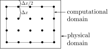
In this course we focus exclusively on the dry-node group: it is easier to implement and retains second-order accuracy as long as the physical wall is placed exactly halfway between two node rows (Krüger et al. 2017). With dry-node boundary conditions, the external contour of the physical domain lies half a cell outside the computational domain, as shown in Figure 1. This is important to remember: evaluating simulated quantities on the physical boundary requires extrapolation of the results, as we will see, for example, for the no-slip wall condition.
Periodic boundary conditions
Periodic boundary conditions implement translational symmetry: fluid that leaves the domain through one boundary re-enters through the opposite one. The condition is typically implemented implicitly during the streaming step, by wrapping the lattice index around at the domain edges.
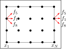
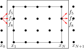
Only the channels that actually cross the boundary are affected. Consider periodicity in the \(x\)-direction with node columns \(x_1, \ldots, x_N\), using the notation of Figure 2. The channels pointing right (\(i \in \{1, 5, 8\}\), see Table 1) leave through the right boundary at \(x_N\) and re-enter at the left boundary \(x_1\): \[ \begin{aligned} f_1(x_1, y, t+\Delta t) &= f_1^{\star}(x_N, y, t), \\ f_5(x_1, y+\Delta y, t+\Delta t) &= f_5^{\star}(x_N, y, t), \\ f_8(x_1, y-\Delta y, t+\Delta t) &= f_8^{\star}(x_N, y, t), \end{aligned} \tag{1}\] where the diagonal channels 5 and 8 additionally shift by one node in the \(y\)-direction, exactly as in ordinary streaming. The analogous relations hold for the channels pointing left (\(i \in \{3, 6, 7\}\)), which leave at \(x_1\) and re-enter at \(x_N\). All other channels are untouched by the boundary.
This condition applies, for example, at the inlet/outlet of a Couette flow, where the flow is driven by the movement of one of the two walls (through the moving-wall condition described below).
Rigid wall: bounce-back
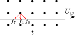
The presence of a rigid wall is modeled by bouncing back the populations that would stream into the wall. Consider the lower wall of a 2D geometry (Figure 3 and Figure 4): after streaming, the upward channels \(f_2\), \(f_5\) and \(f_6\) at the boundary nodes are unknown, since they would have to come from nodes inside the wall. They are determined by assuming that the populations of the downward channels \(f_4\), \(f_7\) and \(f_8\), which leave towards the wall at time \(t\), are reflected by the wall and arrive back in the opposite channels of the same node within one time step \(\Delta t\).
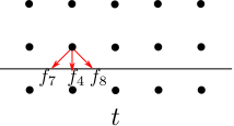
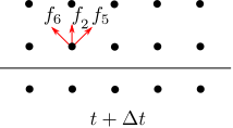
More generally, a population that leaves the boundary node \(\mathbf{x}_b\) at time \(t\) hits the wall (located halfway along the link) and arrives in the opposite channel of the same boundary node at time \(t + \Delta t\). For these populations, the streaming operation is replaced by \[ f_{\bar{i}}(\mathbf{x}_b, t+\Delta t) = f_i^{\star}(\mathbf{x}_b, t), \tag{2}\] where \(\bar{i}\) denotes the channel opposite to \(i\) (Table 1) and \(f^{\star}\) is the pre-streaming (post-collision) value. For example, at the lower wall \[ f_{6}(\mathbf{x}_b, t+\Delta t) = f_{8}^{\star}(\mathbf{x}_b, t), \tag{3}\] since channel 8 points down-right and its opposite, channel 6, points up-left. The bounce-back rule realizes a no-slip condition with the physical wall located halfway between the boundary node and the wall nodes — this is the condition you will use for the stationary walls in milestone 5.
Moving wall
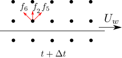
If the wall moves, the bounced-back populations gain or lose momentum during their interaction with the wall. This is described by adding a correction term to the rigid-wall rule of Equation 2 that is proportional to the wall velocity \(\mathbf{u}_w\) (Krüger et al. 2017): \[ f_{\bar{i}}(\mathbf{x}_b, t+\Delta t) = f_i^{\star}(\mathbf{x}_b, t) - 2 w_i \rho_w \frac{\mathbf{c}_i \cdot \mathbf{u}_w}{c_s^2}, \tag{4}\] where \(c_s^2 = 1/3\) is the squared lattice speed of sound in lattice units and the subscript \(w\) denotes quantities evaluated at the wall. Since the wall lies between lattice nodes, the density \(\rho_w\) has to be extrapolated from the bulk, or simply assumed equal to the average density \(\bar{\rho}\).
In Equation 4 the wall velocity is a general vector \(\mathbf{u}_w\). In this course, however, we only consider walls that move parallel to their own surface, as shown in Figure 5 and Figure 6, since this guarantees mass conservation.
As with the rigid wall, \(\bar{i}\) denotes the channel opposite to \(i\) and \(f^{\star}\) the pre-streaming value. The example of Equation 3 becomes \[ f_{6}(\mathbf{x}_b, t+\Delta t) = f_{8}^{\star}(\mathbf{x}_b, t) - 2 w_8 \rho_w \frac{\mathbf{c}_8 \cdot \mathbf{u}_w}{c_s^2}. \tag{5}\]
In the lid-driven cavity of milestone 5, the two top corner nodes belong to both a stationary side wall and the moving lid, so the boundary rules overlap there. Standard practice is either to treat the corner nodes with plain bounce-back (as part of the stationary walls) and apply the moving-wall correction of Equation 4 only along the interior of the lid, or to apply bounce-back with the lid velocity at the two top corners as well. At the low Mach numbers we simulate, any consistent choice gives essentially the same flow field — pick one and document it in your code.
Periodic boundary conditions with a pressure gradient
Periodic boundary conditions can also be used in the presence of a prescribed pressure difference \(\Delta p\) between outlet and inlet. This is the typical situation of flow through a pipe driven by the difference between the inlet pressure \(p_\text{in}\) and the outlet pressure \(p_\text{out}\). The boundary condition reads \[ \begin{aligned} p(\mathbf{x}, t) &= p(\mathbf{x} + \mathbf{L}, t) + \Delta p, \\ \mathbf{u}(\mathbf{x}, t) &= \mathbf{u}(\mathbf{x} + \mathbf{L}, t), \end{aligned} \tag{6}\] where \(\mathbf{L}\) is the domain length along the flow direction. In the lattice Boltzmann method the pressure is directly related to the density through the ideal-gas equation of state3 \[ p = c_s^2 \rho, \tag{7}\] with \(c_s^2 = 1/3\) in lattice units. We are therefore actually imposing \[ \begin{aligned} \rho(\mathbf{x}, t) &= \rho(\mathbf{x} + \mathbf{L}, t) + \Delta \rho, \\ \mathbf{u}(\mathbf{x}, t) &= \mathbf{u}(\mathbf{x} + \mathbf{L}, t), \end{aligned} \tag{8}\] with \(\Delta \rho = \Delta p / c_s^2\).
From the computational point of view, we add an extra layer of nodes outside the physical domain, as shown in Figure 7. If we think of the periodic condition as many identical pipes connected one after another, the extra node column \(x_0\) at the inlet corresponds to the last column \(x_N\) inside the physical domain of the previous pipe, and likewise \(x_{N+1}\) corresponds to the first column \(x_1\) of the next pipe.
The condition is applied to the probability density function, which we decompose into an equilibrium contribution \(f_i^\text{eq}(\rho, \mathbf{u})\) and a non-equilibrium contribution \(f_i^\text{neq}\). The non-equilibrium part is computed before streaming, \[ f_i^\text{neq} = f_i^{\star} - f_i^\text{eq}. \tag{9}\] On the extra nodes we prescribe the equilibrium part with the target density but the velocity of the image node, \[ \begin{aligned} f_i^\text{eq}\big|_{x_0} &= f_i^\text{eq}(\rho_\text{in}, \mathbf{u}_N), \\ f_i^\text{eq}\big|_{x_{N+1}} &= f_i^\text{eq}(\rho_\text{out}, \mathbf{u}_1), \end{aligned} \tag{10}\] while the non-equilibrium part is copied from the corresponding image node. Together, the pre-streaming populations on the extra nodes are \[ \begin{aligned} f_i^{\star}(x_0, y, t) &= f_i^\text{eq}(\rho_\text{in}, \mathbf{u}_N) + \left[ f_i^{\star}(x_N, y, t) - f_i^\text{eq}(x_N, y, t) \right], \\ f_i^{\star}(x_{N+1}, y, t) &= f_i^\text{eq}(\rho_\text{out}, \mathbf{u}_1) + \left[ f_i^{\star}(x_1, y, t) - f_i^\text{eq}(x_1, y, t) \right], \end{aligned} \tag{11}\] with \(\rho_\text{out} = p_\text{out}/c_s^2\) and \(\rho_\text{in} = (p_\text{out} + \Delta p)/c_s^2\). Here \(\mathbf{u}_N\) and \(\mathbf{u}_1\) denote the velocities at the image nodes \(x_N\) and \(x_1\). The ordinary streaming step then transports these populations into the domain; only the channels that actually stream inward matter (\(i \in \{1, 5, 8\}\) from \(x_0\), and \(i \in \{3, 6, 7\}\) from \(x_{N+1}\)).
Inlet
There are several ways to implement an inlet condition; here we describe the most direct approach, which assigns a velocity and density profile at the inlet. The inlet velocity \(\mathbf{u}_\text{in}\) and density \(\rho_\text{in}\) are imposed by directly assigning the equilibrium distribution at the boundary node \(\mathbf{x}_b\), \[ f_i(\mathbf{x}_b, t+\Delta t) = f_i^\text{eq}(\rho_\text{in}, \mathbf{u}_\text{in}), \tag{12}\] where \(f_i^\text{eq}\) is the equilibrium distribution function. This assignment replaces the populations after the streaming step, i.e. it overwrites whatever has streamed into the node. Note that this inlet condition has to be applied to all channels \(i\), not only to the channels that point into the domain.
Outlet
We have seen in the previous sections that the unknowns at any boundary are the populations entering the domain. The same holds at an outlet, where we can extrapolate this information from the second-to-last node \(\mathbf{x}_{b2} = \mathbf{x}_b - \Delta\mathbf{x}\) before the boundary node \(\mathbf{x}_b\): \[ f_i(\mathbf{x}_b, t+\Delta t) = f_i^{\star}(\mathbf{x}_{b2}, t), \tag{13}\] where the index \(i\) runs over the channels pointing into the domain (e.g. \(i \in \{3, 6, 7\}\) for an outlet on the right edge, see Table 1) and \(f^{\star}\) again denotes the pre-streaming populations. Equation Equation 13 replaces the streaming step for these channels: the unknown incoming populations are approximated by the corresponding pre-streaming populations one node further inside the domain, which amounts to a zero-gradient assumption at the outlet.
Alternatively, one can use a second-order extrapolation scheme that also exploits the information in the third-to-last node \(\mathbf{x}_{b3} = \mathbf{x}_b - 2\Delta\mathbf{x}\): \[ f_i(\mathbf{x}_b, t+\Delta t) = 2 f_i^{\star}(\mathbf{x}_{b2}, t) - f_i^{\star}(\mathbf{x}_{b3}, t). \tag{14}\]
References
Footnotes
Streaming and collision are also called propagation and relaxation, respectively.↩︎
In the usual implementation, the streaming operation is applied at the boundary nodes as well, and the result is corrected immediately afterwards by a boundary-condition routine.↩︎
To be precise: we simulate the flow of an incompressible fluid with the lattice Boltzmann equation, which is derived for a compressible fluid obeying the ideal-gas equation of state.↩︎