Chapter 8
Discrete convolutions
Context: This chapter revisits the discrete Fourier transform (DFT) and illustrates how it can be used for the efficient computation of cyclic convolutions. Nonlinear terms in partial differential lead to noncyclic convolutions in Fourier spectral methods. Direct application of the DFT then yield aliasing errors, which can be corrected through dealiasing procedures.
8.1 Discrete Fourier transform
The Fourier series represents functions on finite domains of length \(L\) as \begin {equation} f(x) = \frac {1}{L} \sum _{n=-\infty }^\infty \tilde {f}(q_n) \exp \left (i q_n x\right ) \label {eq:fourier-series} \end {equation} with \(q_n=2\pi n/L\). The inverse transform is given by \begin {equation} \tilde {f}(q_n) = \int _0^L \dif x\, f(x) \exp \left (-i q_n x\right ). \label {eq:inverse-fourier-series} \end {equation} We now evaluate the Fourier series only on discrete, equidistant sampling points \(x_k=kL/N\). The inverse transform Eq. \eqref{eq:inverse-fourier-series} then becomes \begin {equation} \tilde {f}(q_n) = \frac {L}{N} \sum _{k=0}^{N-1} f(x_k) \exp \left (-i q_n x_k\right ), \end {equation} where the sum is the discrete variant of \(\int \dif x\approx \sum \Delta x\) with grid spacing \(\Delta x=L/N\). The phase-factor \(q_n x_k = 2\pi kn/N\) is an integer multiple of \(2\pi \) if \(n\) is an integer multiple of \(N\), hence \(\tilde {f}(q_{n+\alpha N})=\tilde {f}(q_{n})\) because \(k(n+\alpha N)/N=kn/N + k\alpha \) for integer \(\alpha \in \mathbb {Z}\). Formally this means that Eq. \eqref{eq:fourier-series} diverges. This is consistent with the interpretation that the discretely sampled \(f(x_k)\) is a convolution of \(f(x)\) with a Dirac comb. We can truncate the forward transform to \begin {equation} f(x_k) = \frac {1}{L} \sum _{n=M}^{M+N-1} \tilde {f}(q_n) \exp \left (i q_n x_k\right ) = \sum _{n=M}^{M+N-1} W_{kn} \hat {f}_n , \label {eq:discrete-fourier-transform} \end {equation} where \(\hat {f}_n=\tilde {f}(q_n)/L\) and we are using the DFT-matrix \(W_{kn}=\exp (i 2\pi k n/N)\), see also Eq. \eqref{eq:dft-matrix}. This indeed yields the correct discretely sampled function, as can be seen by inserting the inverse transform Eq. \eqref{eq:inverse-discrete-fourier-transform} into Eq. \eqref{eq:discrete-fourier-transform}. The choice of \(M\in \mathbb {Z}\) in Eq. \eqref{eq:discrete-fourier-transform} remains completely arbitrary, but a typical choice is \(M=0\). Equation \eqref{eq:discrete-fourier-transform} is called the discrete Fourier transform (DFT) with inverse Eq. \eqref{eq:inverse-discrete-fourier-transform} which can be rewritten to \begin {equation} \hat {f}_n = \frac {1}{N} \sum _{k=0}^{N-1} W_{nk}^* f(x_k). \label {eq:inverse-discrete-fourier-transform} \end {equation} The DFT is typically computed using a fast Fourier transform algorithm (FFT), that reduces the computational complexity from \(O(N^2)\) of a naive implementation of Eq. \eqref{eq:discrete-fourier-transform} to \(O(N \log N)\).
8.2 Cyclic convolutions
The FFT is useful to reduce the complexity of computing cyclic convolutions from \(O(N^2)\) to \(O(N \log N)\). A cyclic convolution of the discrete series \(a_n\) and \(b_n\) is given by \begin {equation} c_k = \sum _{n=0}^{N-1} a_n b_{A(k-n)} \end {equation} where \(A(m)=m+\alpha N\) with \(\alpha \in \mathbb {Z}\) such that \(0\leq A(m)<N\). We can insert the DFT expression, Eq. \eqref{eq:discrete-fourier-transform}, which automatically fulfills the cyclic property to obtain \begin {equation} \begin {split} c_k &= \frac {1}{N^2} \sum _{n=0}^{N-1} \sum _{m=0}^{N-1} W_{nm} \hat {a}_m \sum _{l=0}^{N-1} W_{k-n,l} \hat {b}_l \\ &= \frac {1}{N^2} \sum _{m=0}^{N-1} \sum _{l=0}^{N-1} \hat {a}_m W_{kl} \hat {b}_l \sum _{n=0}^{N-1} W_{n,m-l} \\ &= \frac {1}{N^2} \sum _{m=0}^{N-1} \sum _{l=0}^{N-1} \hat {a}_m W_{kl} \hat {b}_l N\delta _{m,l} \\ &= \frac {1}{N} \sum _{m=0}^{N-1} W_{km} \hat {a}_m \hat {b}_m, \end {split} \end {equation} which is the discrete Fourier transform representation of the product, i.e. \begin {equation} \hat {c}_m=\hat {a}_m\hat {b}_m. \label {eq:cyclic-convolution-dft} \end {equation} This means the convolution requires an element-wise product with complexity \(O(N)\), plus three fast Fourier transforms, which all have complexity \(O(N\log N)\).
8.3 Nonlinear terms and aliasing
We now discuss the treatment of nonlinear terms in numerical solution of partial differential equations with Fourier spectral methods. As an example, let us regard the simple multiplication of two functions, \begin {equation} h(x) = f(x) g(x). \label {eq:nonlinear-example} \end {equation} We expand both \(f(x)\), \(g(x)\) and \(h(x)\) into a truncated Fourier series, i.e. we write \begin {align} f(x) &\approx \sum _{n=-N}^N \hat {a}_n \exp \left (iq_nx\right ), \\ g(x) &\approx \sum _{m=-N}^N \hat {b}_m \exp \left (iq_mx\right ), \\ h(x) &\approx \sum _{k=-N}^N \hat {c}_k \exp \left (iq_kx\right ).\label {eq:h_orginal_range} \end {align}
To simplify notation, we use \(N\) to denote the truncation of the sums which now run over \(2N+1\) terms.
Inserting into Eq. \eqref{eq:nonlinear-example} yields \begin {equation} h(x) = \sum _{n=-N}^N \sum _{m=-N}^N \hat {a}_n \hat {b}_m \exp \left (iq_{n+m}x\right ). \end {equation} This means, that \(h(x)\) is expressed as a truncated Fourier series with frequencies \(q_{n+m}\) from range \(-2N\leq n+m \leq 2N\). However, we can expand \(h(x)\) in the original range of frequencies from Eq. \eqref{eq:h˙orginal˙range} as follows.
The discrete form of this equation can be obtained from the Galerkin method, i.e. by multiplying with \(\exp \left (iq_kx\right )\) from the left, which yields \begin {equation} \hat {c}_k = \frac {1}{L} \left (\exp (iq_kx), h(x)\right ) = \sum _{n=-N}^N \sum _{m=-N}^N \hat { a}_n \hat {b}_m \delta _{k,n+m} = \sum _{n=-N}^N \hat { a}_n \hat {b}_{k-n}, \label {eq:nonlinear-convolution} \end {equation} and thus \begin {equation} h(x) = \sum _{k=-N}^N \underbrace { \sum _{n=-N}^N \hat { a}_n \hat {b}_{k-n}}_{\hat {c}_k} \exp \left (iq_{k}x\right ). \end {equation} An important observation is that \(\hat {c}_k\) is nonzero in the range \(-2N\leq k \leq 2N\), but we truncated the sum at \(N\). Since \(\hat {b}_m\) in Eq. \eqref{eq:cyclic-convolution-dft} is not cyclic, using the discrete Fourier transform to compute this convolution introduces an error. This type of numerical error is called aliasing.
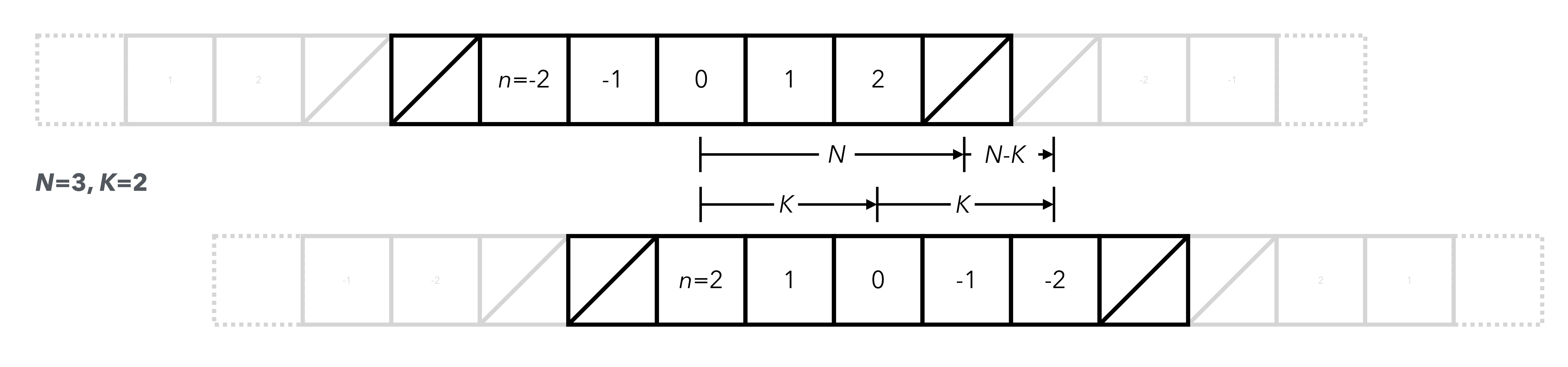
Aliasing can be removed from the cyclic convolution by zero padding the two vectors. We set \(\hat {a}_n=0\) and \(\hat {b}_n=0\) for \(n > K\). The value of \(\hat {c}_k\) is then exact for \(k\leq K\) if \(2K\leq N+(N-K)\), yielding \(K\leq 2N/3\) (see Fig. 8.1 for an illustration). This means we can compute the convolution, Eq. \eqref{eq:nonlinear-convolution}, using the FFT for the cyclic convolution at the expanse of discarding \(1/3\) of the wavevectors. This is called the \(2/3\) rule (Orszag, 1971).