Tutorial 1: Playing with the Fourier transform

Although we have (likely) not yet discussed details of the Fourier transform in the lecture, we would like to start playing a bit with it to get an intuitive understanding of what it does. The Fourier transform decomposes a function into contributions from different wavelength. The function is then given by the sum of sine and cosine contributions. When we talk about Fourier transform in the context of these exercise sheet, we mean the discrete Fourier transform as typically compute using a fast-Fourier transforms (FFT) algorithm.

One-dimensional transforms

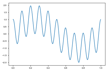
We will here look at how the Fourier transform decomposes the signal into individual contributions. We will start with a function that is given by the sum of two sine waves:

%matplotlib inline
import numpy as np
import matplotlib.pyplot as plt
x = np.linspace(0, 1, 1000)
f = np.sin(2*np.pi*x) + np.cos(2*np.pi*10*x)
plt.plot(x, f)

[<matplotlib.lines.Line2D at 0x118d4f198>]

png

Task 1

Check the documentation of the numpy.fft module to understand what the FFT computes. Compute the transform of the above function. Note that the Fourier transform yields a complex number that has real and imaginary parts, or equivalently, an amplitude and a phase. Plot only the amplitude or the square of the amplitude of the above function as a function of wavevector. (What is a wavevector? You get hints at this by reading the documentation. Also look at the documentation of the helper function numpy.fft.fftfreq.) The square of the amplitude is also called the power spectrum of that function. What do you see?

Task 2

Remove all wavelengths smaller than $0.3$. Compute and plot the inverse transform the function. What do you see and why?

Two-dimensional transforms

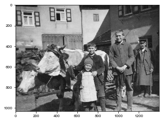
Use opencv to load the image Picture.jpg provided in this folder. An example on how to use opencv to load and display an image follows.

Hint:

You may need to install opencv from the commandline using python3 -m pip install --user opencv-python.

import cv2
img = cv2.imread('Picture.jpg', 0)
plt.imshow(img, cmap='gray')

<matplotlib.image.AxesImage at 0x12155cc88>

png

Task 1

Plot the power spectrum of the above image. It can be useful to use the function numpy.fftshift and/or numpy.ifftshift to shift the zero wavevector components to the center of the image.

Task 2

Successively remove the long wavelength contribution to the image. Compute the inverse FFT and display the image again. What do you see and why?