Kinematics and constraints
After completing this chapter, you should be able to:
- Construct rotation matrices and apply them for coordinate transformations
- Calculate the velocity of any point on a rigid body using \(\vec{v}_P = \vec{v}_O + \vec{\omega} \times \vec{r}_{P/O}\)
- Determine degrees of freedom and whether a structure is movable, isostatic, or hyperstatic
Rigid-body kinematics
Every rigid body motion in 3D space is a composition of translations and rotations. Why translations are trivial, we need to discuss rotations in detail.
Rotation matrix
A rotation \(\mathcal{R}\) is a linear operation that does not affect the length (or norm) of the vector, \(|\mathcal{R}\vec{x}|=|\vec{x}|\). We distinguish between the operation \(\mathcal{R}\) and its representation in the form of a matrix \(\underline{R}\) (we use underlines to denote matrices and second-order tensors throughout these notes). We can write the rotation as the product of this matrix with a vector, \[|\underline{R}\cdot \vec{x}| = ( R_{ij} x_j R_{ik} x_k )^{1/2} = ( x_j R^T_{ji} R_{ik} x_k )^{1/2} = \left ( \vec{x}\cdot \underline{R}^T\cdot \underline{R}\cdot \vec{x} \right )^{1/2}. \] This must be equal equal to \(|\vec{x}|\), which implies \(\underline{R}^T\cdot \underline{R}=\underline{I}\), i.e. if the rotation matrix \(\underline{R}\) is an orthogonal matrix. Here the superscript \(^T\) indicates the transpose operation, \(R^T_{ij}=R_{ji}\), and \(\underline{I}\) is the unit matrix. Note that this relationship implies \(\underline{R}^{-1}=\underline{R}^T\), i.e. the inverse of an orthogonal matrix is simply its transpose.
Let us assume we want to rotate from a coordinate system with basis vectors \(\hat {x}\), \(\hat {y}\), and \(\hat {z}\) to a primed coordinate system \(\hat {x}'\), \(\hat {y}'\), and \(\hat {z}'\). The rotation operator \(\mathcal{R}\) should transform the basis vectors of the unprimed into the primed system, \[\mathcal{R}\hat {x} = \hat {x}', \quad \mathcal{R}\hat {y} = \hat {y}', \quad \mathcal{R}\hat {z} = \hat {z}'. \] We can construct the rotation matrix from this definition of the action of the rotation on the basis vectors. From the component definition we obtain \[\underline{R} = \begin {pmatrix} R_{xx} & R_{xy} & R_{xz} \\ R_{yx} & R_{yy} & R_{yz} \\ R_{zx} & R_{zy} & R_{zz} \end {pmatrix} = \begin {pmatrix} \hat {x}\cdot \mathcal{R}\hat {x} & \hat {x}\cdot \mathcal{R}\hat {y} & \hat {x}\cdot \mathcal{R}\hat {z} \\ \hat {y}\cdot \mathcal{R}\hat {x} & \hat {y}\cdot \mathcal{R}\hat {y} & \hat {y}\cdot \mathcal{R}\hat {z} \\ \hat {z}\cdot \mathcal{R}\hat {x} & \hat {z}\cdot \mathcal{R}\hat {y} & \hat {z}\cdot \mathcal{R}\hat {z} \end {pmatrix} = \begin {pmatrix} \hat {x}\cdot \hat {x}' & \hat {x}\cdot \hat {y}' & \hat {x}\cdot \hat {z}' \\ \hat {y}\cdot \hat {x}' & \hat {y}\cdot \hat {y}' & \hat {y}\cdot \hat {z}' \\ \hat {z}\cdot \hat {x}' & \hat {z}\cdot \hat {y}' & \hat {z}\cdot \hat {z}' \end {pmatrix}. \] If all vectors are expressed in the coordinate system \(\{\hat {x}, \hat {y}, \hat {z}\}\), then the rotation matrix can be written as \[\underline{R} = (\hat {x}', \hat {y}', \hat {z}'), \] i.e. by stacking the rotated basis vectors as columns. The matrix \(\underline{R}\) is orthogonal, since \[\underline{R}^T\cdot \underline{R} = \begin {pmatrix} \hat {x}'\cdot \hat {x}' & \hat {x}'\cdot \hat {y}' & \hat {x}'\cdot \hat {z}' \\ \hat {y}'\cdot \hat {x}' & \hat {y}'\cdot \hat {y}' & \hat {y}'\cdot \hat {z}' \\ \hat {z}'\cdot \hat {x}' & \hat {z}'\cdot \hat {y}' & \hat {z}'\cdot \hat {z}' \end {pmatrix} = \underline{I}, \] if \(\{\hat {x}', \hat {y}', \hat {z}'\}\) form an orthonormal triad.
For example, a counterclockwise rotation by an angle \(\theta\) about the \(z\)-axis leaves \(\hat {z}\) unchanged: \[\hat {x}' = \begin {pmatrix} \cos \theta \\ \sin \theta \\ 0 \end {pmatrix}, \quad \hat {y}' = \begin {pmatrix} -\sin \theta \\ \cos \theta \\ 0 \end {pmatrix}, \quad \hat {z}' = \begin {pmatrix} 0 \\ 0 \\ 1 \end {pmatrix}. \] The corresponding rotation matrix is \[\label {eq:rotmat3D} \underline{R}_z(\theta ) = \begin {pmatrix} \cos \theta & -\sin \theta & 0 \\ \sin \theta & \cos \theta & 0 \\ 0 & 0 & 1 \end {pmatrix}. \] It is straightforward to verify that \(\underline{R}_z^T \underline{R}_z = \underline{1}\) and \(\det (\underline{R}_z) = 1\).
Similarly, rotations about the \(x\)- and \(y\)-axes are given by \[\begin{align} \underline{R}_x(\theta ) &= \begin {pmatrix} 1 & 0 & 0 \\ 0 & \cos \theta & -\sin \theta \\ 0 & \sin \theta & \cos \theta \end {pmatrix}, \\[6pt] \underline{R}_y(\theta ) &= \begin {pmatrix} \cos \theta & 0 & \sin \theta \\ 0 & 1 & 0 \\ -\sin \theta & 0 & \cos \theta \end {pmatrix}. \end{align}\]
Coordinate transformation of a vector
One function of the rotation matrix is to change the coordinate of a vector from one reference system to another one. Let \(\vec{p}\) be the position vector of a point in three-dimensional space. Its representation in the unprimed coordinate system is given by the components \[\vec{p} = p_x \, \hat {x} + p_y \, \hat {y} + p_z \, \hat {z}. \] After a rotation of the coordinate system, the same point can be expressed in the primed basis as \[\vec{p'} = p_x' \, \hat {x}' + p_y' \, \hat {y}' + p_z' \, \hat {z}'. \] Since \(\hat {x}'\), \(\hat {y}'\), and \(\hat {z}'\) are related to the original basis vectors by the rotation matrix \(\underline{R}\), \[\begin {pmatrix} \hat {x}' & \hat {y}' & \hat {z}' \end {pmatrix} = \begin {pmatrix} \hat {x} & \hat {y} & \hat {z} \end {pmatrix} \underline{R}, \] we can write the same vector in component form as \[\begin {pmatrix} \hat {x} & \hat {y} & \hat {z} \end {pmatrix} \vec{p} = \begin {pmatrix} \hat {x}' & \hat {y}' & \hat {z}' \end {pmatrix} \vec{p'}. \] Equating the two expressions gives \[\vec{p} = \underline{R} \, \vec{p'}, \quad \text {or equivalently} \quad \vec{p'} = \underline{R}^T \, \vec{p}. \] That is, the rotation matrix \(\underline{R}\) transforms the basis vectors (a passive rotation), while its transpose \(\underline{R}^T\) transforms the coordinate components of the position vector between the two reference frames.
As an example, for a rotation about the \(z\)-axis by an angle \(\theta\), \[\vec{p'} = \underline{R}_z^T(\theta ) \vec{p} = \begin {pmatrix} \cos \theta & \sin \theta & 0 \\ -\sin \theta & \cos \theta & 0 \\ 0 & 0 & 1 \end {pmatrix} \begin {pmatrix} p_x \\ p_y \\ p_z \end {pmatrix}. \]Thus the components in the rotated coordinate system are \[\begin{align} p_x' &= p_x \cos \theta + p_y \sin \theta , \\ p_y' &= -p_x \sin \theta + p_y \cos \theta , \\ p_z' &= p_z. \end{align}\]
Differentiation of the rotation matrix
A rotation matrix \(\underline{R}(t)\) in three-dimensional space describes the orientation of a rotating coordinate frame as a function of time. By definition, a rotation matrix is orthogonal and has unit determinant: \[\underline{R}(t)\underline{R}(t)^T = \underline{I}, \quad \det \underline{R}(t) = 1. \] Differentiating the orthogonality condition with respect to time yields \[\dot {\underline{R}}(t)\underline{R}(t)^T + \underline{R}(t)\dot {\underline{R}}(t)^T = \underline{0}. \tag{1}\] This equation expresses the fact that the product \(\dot {\underline{R}}(t)\underline{R}(t)^T\) is skew-symmetric. Indeed, multiplying Equation 1 from the right by \(\underline{R}(t)\) gives \[\dot {\underline{R}}(t) = \underline{\Omega }(t)\underline{R}(t), \] where we define \[\underline{\Omega }(t) = \dot {\underline{R}}(t)\underline{R}(t)^T. \] Taking the transpose, \[\underline{\Omega }(t)^T = \underline{R}(t)\dot {\underline{R}}(t)^T, \] so that \(\underline{\Omega }(t)\) is a skew-symmetric matrix, since
\[\underline{\Omega }(t) + \underline{\Omega }(t)^T = \underline{0}. \] Now, a \(3\times 3\) skew-symmetric matrix has only three independent components, which can be associated with the components of the angular velocity vector \(\vec{\omega}(t)\). We therefore write \[\underline{\Omega }(t) = \begin {pmatrix} 0 & -\omega _z & \omega _y \\ \omega _z & 0 & -\omega _x \\ -\omega _y & \omega _x & 0 \end {pmatrix}, \tag{2}\] such that for any vector \(\vec{p}\), \[\underline{\Omega }(t)\vec{p} = \vec{\omega }(t) \times \vec{p}. \tag{3}\] This matrix form provides a compact representation of the cross product operation.
Thus, the time evolution of the rotation matrix is governed by the first-order matrix differential equation \[\dot {\underline{R}}(t) = \underline{\Omega}(t)\underline{R}(t), \tag{4}\] where \(\underline{\Omega }(t)\) is constructed from the instantaneous angular velocity vector \(\vec{\omega}(t)\).
Relative velocity
Consider a rigid body with a body-fixed coordinate frame whose orientation and position relative to an inertial (world) frame are given by a time-dependent rotation matrix \(\underline{R}(t)\) and a translation (origin) vector \(\vec{r}_O(t)\). Let \(\vec{p}\) denote the coordinates of a material point in the body frame (constant in time for the rigid body assumption), and let \(\vec{r}_P(t)\) be the position of that same point expressed in the world frame. The kinematic relation between these is \[\vec{r}_P(t) = \vec{r}_O(t) + \underline{R}(t)\,\vec{p}. \tag{5}\] Differentiate Equation 5 with respect to time to obtain the point velocity in the world frame: \[\vec{v}_P(t) = \vec{v}_O(t) + \dot {\underline{R}}(t)\,\vec{p}. \tag{6}\] Using the angular-velocity matrix \(\underline{\Omega }(t)\) defined by \[\underline{\Omega }(t) = \dot {\underline{R}}(t)\underline{R}(t)^T,\] we can express \(\dot {\underline{R}}(t)\) as \(\dot {\underline{R}}(t)=\underline{\Omega }(t)\underline{R}(t)\). Substitute this into Equation 6: \[\vec{v}_P(t) = \vec{v}_O(t) + \underline{\Omega }(t)\underline{R}(t)\,\vec{p}. \]But \(\underline{R}(t)\vec{p} = \vec{r}_P(t) - \vec{r}_O(t) = \vec{r}_{P/O}\) from Equation 5,
so \[\vec{v}_P(t) = \vec{v}_O(t) + \underline{\Omega }(t)\vec{r}_{P/O}. \tag{7}\] Recall that \(\underline{\Omega}(t)\) is skew-symmetric and can be associated with the angular velocity vector \(\vec{\omega }(t)\) as per Equation 4.
Thus Equation 7 becomes the familiar rigid-body velocity rule \[\boxed {\; \vec{v}_P(t) \;=\; \vec{v}_O(t) \;+\; \vec{\omega }(t) \times \vec{r}_{P/O}\;} \tag{8}\] or, in words: the velocity of any point equals the velocity of the chosen reference point (origin of the body frame) plus the instantaneous angular velocity cross the vector from that reference point to the point considered.
Constraints and degrees of freedom
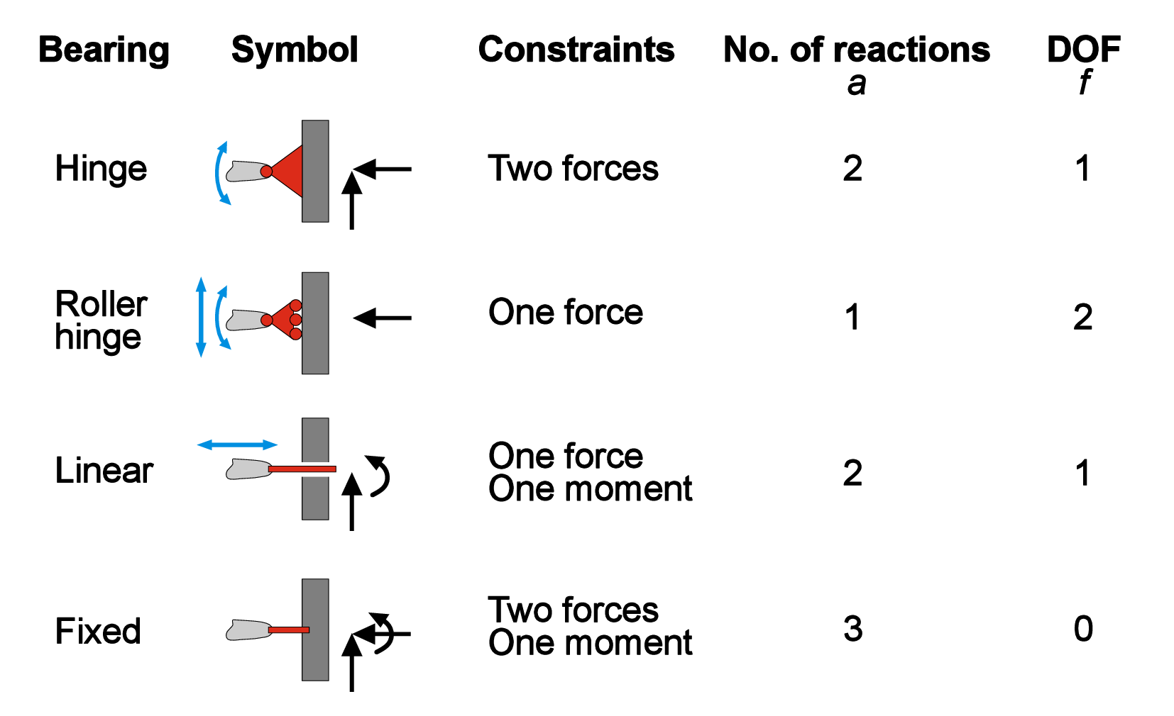
The condition of static equilibrium that we discussed in Chapter 1 does not mean that the body is immovable. As you saw in the previous section, the body still can translate and rotate; in a two-dimensional case an object can have three kinematics degrees of freedom (DoFs): two orthogonal translational displacements along x- and y- axes, and one rotation around z-axis. The motion of the body can be constrained by eliminating some DoFs with the help of supports (Figure 1). Depending on the type of support, one, two, or all three DoFs can be removed. The kinematic constraints imposed by supports trigger so-called reaction forces, or simply reactions. Note that if exactly all degrees of freedom are removed, the system is called statically determinate or isostatic.
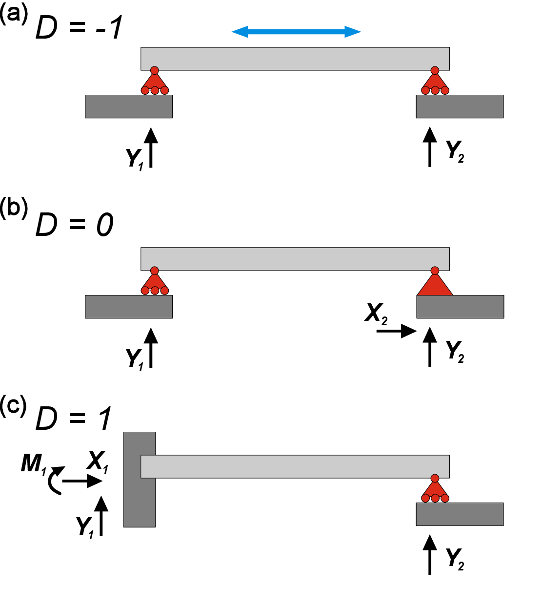
As you can see, the sum of the degrees of constraints \(c_i\) and DoFs \(f_i\) is always equal to 3 (for 2D case). This is a necessary (but not a sufficient!) condition for a statically determinate system with one body and \(m\) constraints. Namely, \[3-\sum _{i}^{m}{c_i}=0 \]For more general 2D system with \(n\) connected bodies \[3n-\sum _{i}^{m}{c_i}=0. \] By having \(n\) bodies, \(m\) constraints of degree \(c_i\), we can distinguish three different cases for 2D force systems defined by the value of \(D\), where \[D=3n-\sum _{i}^{m}{c_i} \label {eq:D} \]We know that a determinate (or isostatic) system must have \(D=0\) (Figure 2 b). If \(D>0\), then the system is movable or kinematically indeterminate since it has unrestricted DoF (Figure 2 a). If \(D<0\), then the system is called statically indeterminate or hyperstatic - the system is immovable and contains extra reactions that can be removed (Figure 2 c).
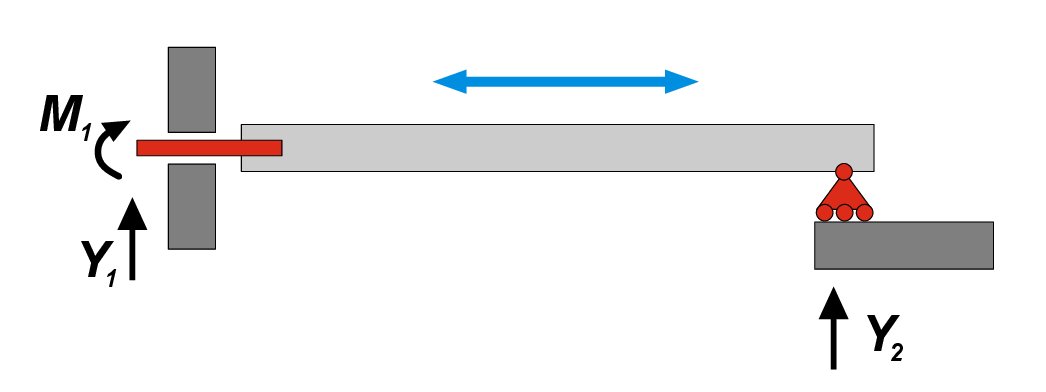
Again, we need to emphasize that above-mentioned mathematical precondition is a necessary, but not sufficient, requirement. One exception from this rule is the system with two and one reactions in the left and right supports respectively shown in Figure 3. Here, we have \(D=0\), which usually corresponds to determinate system. However, it is clear that the beam can move freely in a horizontal direction, therefore it has 1 DoF! In this specific case, force vectors \(Y_1\) and \(Y_2\) are parallel, and they both can compensate only vertical direction of action, while the horizontal movement is not restricted. It means that the constraints are ill placed. A systematic way to determine if constraints are well placed consists in determining the Instantaneous Center of Rotation.
Instantaneous Center of Rotation.
In planar (2D) kinematics, the Instantaneous Center of Rotation \(C\) is a point in or outside a rigid body about which the entire body appears to rotate at a given instant of time.
At that instant, all points of the body have velocities that are equivalent to those of a pure rotation about the \(C\).
Consider a rigid body moving in a plane. At any instant, the motion can be described as a combination of translation and rotation. The instantaneous center of rotation is defined as the point of the body (or its extension) that has zero velocity at that instant. \[v_{C} = 0\] All other points of the body move as if rotating about this point.
Let the body have an angular velocity $$ (positive counterclockwise). If \(P\) is a point on the body and \(r_{P/C}\) is the position vector from the \(C\) to \(P\), the velocity of \(P\) is given by \[\vec{v}_P = \vec{\omega } \times \vec{r}_{P/C}\] In planar motion, this reduces to the scalar relation: \[v_P = \omega \, r_{P/C}\] where \(r_{P/C}\) is the distance between \(P\) and the instantaneous center.
If the instantaneous center of rotation is located at infinity, the motion is a pure translation without rotation (if \(r_{P/C} \to \infty\) then $ $).
Thus, given an assembly of rigid bodies, it is appropriate to verify the existence of \(C\) in order to determine if a structure is really static (\(D\le 0\)) or if some constraints are ill placed, as in the example of Figure 3.
The existence of \(C\) can be determined by looking at the constraints. Single constraints allow for infinite possible centers of rotations: all the points of the line perpendicular to the direction of motion of the roller, and all the points at the infinity for the rotation lock. Double constraints allow only one center of rotations: the center of the hinge or the point at the infinity in the direction perpendicular to the movement of the linear bearing. Triple constraints do not allow any possible center of rotation.
For a single constrained rigid body, if there is a point in common among all possible instantaneous centers of rotations of each constraint, that point is \(C\) and
the body is kinematically indeterminate. For example, in the structure depicted in Figure 3, the linear bearing admits only one possible \(C\) at the infinity, in the direction perpendicular to axis of the beam, and the roller allows infinite ICRs normal to the roller, including of course the point at the infinity. Thus, both constraints admit \(C\) at the infinity perpendicular to the beam, which is indeed the point around which the beam can freely rotate (i.e. the beam can translate rigidly horizontally).
When moving from a single beam to systems of rigid bodies, it becomes necessary to distinguish between different definitions of the instantaneous center of rotation:
The absolute center of rotation, denoted as \(C_i\), is the point around which the \(i\)-th body rotates. This point is therefore fixed with respect to a global reference system, and its existence is only possible in mechanisms that are kinematically undetermined and statically impossible (\(D>0\)).
The relative center of rotation between two bodies is the point \(C_{ij}\) such that, when observing body \(i\) from a reference frame attached to body \(j\), the latter would appear to be at rest while the former rotates about \(C_{ij}\). External constraints affect the position of the absolute center, while internal constraints affect that of the relative center, in a way entirely analogous to what has already been discussed.
For an assembly consisting of two rigid bodies, we can use the first theorem of kinematic chains: given a structure consisting of two rigid bodies \(i\) and \(j\), a necessary and sufficient condition for it to be a mechanism is that the instantaneous centers of rotation \(C_i\), \(C_j\), and \(C_{ij}\) are aligned.
This chapter covered kinematics and structural constraints:
- Rotation matrices: Orthogonal matrices (\(\underline{R}^T\cdot\underline{R}=\underline{1}\)) that represent rotations; constructed by stacking rotated basis vectors as columns
- Angular velocity: The skew-symmetric matrix \(\underline{\Omega}=\dot{\underline{R}}\underline{R}^T\) encodes the angular velocity vector \(\vec{\omega}\)
- Rigid-body velocity rule: \(\vec{v}_P = \vec{v}_O + \vec{\omega} \times \vec{r}_{P/O}\) relates velocities of different points
- Degrees of freedom (DoF): In 2D, a free body has 3 DoFs (two translations, one rotation)
- Supports: Remove DoFs; rollers (1), hinges (2), fixed supports (3)
- Static determinacy: Computed via \(D = 3n - \sum c_i\); \(D=0\) is isostatic, \(D>0\) is movable, \(D<0\) is hyperstatic
- Instantaneous center of rotation (ICR): The point about which a body instantaneously rotates; useful for checking if constraints are properly placed
Understanding kinematics is essential for analyzing both the motion of mechanisms and the stability of static structures.