After completing this chapter, you should be able to:
Define kinematic quantities (\(u\), \(w\), \(\varphi\)) and strain measures (\(\varepsilon\), \(\gamma\), \(\chi\)) for beams
State the Bernoulli hypothesis and derive the Euler-Bernoulli beam equation \(EI w'''' = q\)
Solve beam deflection problems by integrating the beam equation with boundary conditions
We now transition from the study of rigid bodies and internal forces to the kinematics of deformable bodies. In this chapter, we focus on beams, which are one-dimensional structural elements where one dimension (the length along the beam axis) is significantly larger than the other two dimensions (width and height of the cross-section).
The kinematics of beams describes how points in the beam move and deform when subjected to loads. Unlike rigid bodies where deformation is ignored, beam kinematics explicitly accounts for changes in shape and curvature.
Beam geometry and coordinates
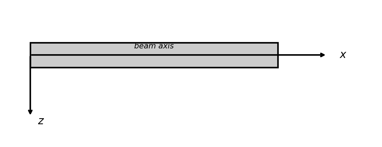
Consider a straight beam of length \(L\) oriented along the \(x\)-axis. The beam has a cross-section in the \(y\)-\(z\) plane, where \(z\) is the direction perpendicular to the beam axis in which bending occurs. We focus on deformation in the \(x\)-\(z\) plane.
Figure 1: Beam geometry showing the coordinate system. The beam extends along the \(x\)-axis with the \(z\)-axis pointing downward.
Figure 1 shows an undeformed beam. The beam axis passes through the centroid of the cross-section. In the undeformed configuration, this axis is a straight line along the \(x\)-direction. We will in the following assume that the beam is a slender object, i.e. we can ignore its finite thickness.
Kinematic quantities
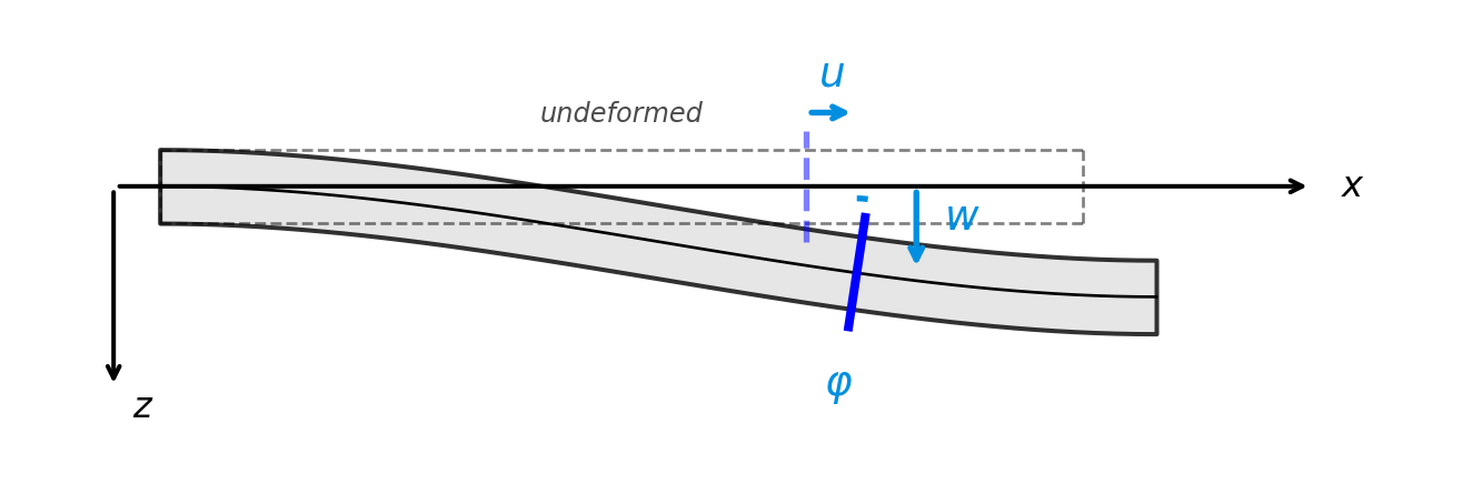
When a beam deforms, we describe its motion using two fundamental displacement quantities measured at the beam axis. The axial displacement\(u(x)\) describes the displacement of the beam axis in the \(x\)-direction. The deflection\(w(x)\) is the displacement of the beam axis in the \(z\)-direction (perpendicular to the beam). In addition to translation, cross-sections of the beam can rotate. We denote the rotation of a cross-section by \(\varphi(x)\), measured positive counterclockwise (i.e., a positive rotation tilts the cross-section such that its top moves in the negative \(x\)-direction). Figure 2 illustrates these quantities.
Code
import numpy as npimport matplotlib.pyplot as pltfrom matplotlib.patches import Rectangle, FancyArrowPatch, Arcimport matplotlib.transforms as transformsfig, ax = plt.subplots(figsize=(7, 3))# Colorsbeam_color ='#cccccc'deformed_color ='#e0e0e0'arrow_color ='#008fe0'# Beam dimensionsL =1.0beam_height =0.08# Draw undeformed beam (dashed outline)ax.plot([0, L], [-beam_height/2, -beam_height/2], 'k--', linewidth=1, alpha=0.5)ax.plot([0, L], [beam_height/2, beam_height/2], 'k--', linewidth=1, alpha=0.5)ax.plot([0, 0], [-beam_height/2, beam_height/2], 'k--', linewidth=1, alpha=0.5)ax.plot([L, L], [-beam_height/2, beam_height/2], 'k--', linewidth=1, alpha=0.5)ax.text(0.5, beam_height/2+0.03, 'undeformed', fontsize=9, ha='center', style='italic', alpha=0.7)# Draw deformed beam (shifted and deflected downward with z pointing down)u_val =0.08# axial displacementw_val =0.12# deflection (positive = downward in z-down convention)# Deformed beam - simple representation with curved axisx_def = np.linspace(0, L, 50)# Cubic deflection shape (negative in plot since z points down but plot y points up)w_def =-w_val * (3*(x_def/L)**2-2*(x_def/L)**3)u_def = u_val * x_def/L# Draw deformed beam outline (approximate)ax.fill_between(x_def + u_def, w_def - beam_height/2, w_def + beam_height/2, facecolor=deformed_color, edgecolor='black', linewidth=1.5, alpha=0.8)# Draw beam axis (deformed)ax.plot(x_def + u_def, w_def, 'k-', linewidth=1)# Mark a specific cross-section locationx_cs =0.7idx =int(x_cs/L *49)x_cs_def = x_cs + u_def[idx]w_cs_def = w_def[idx]# Calculate local rotation at this point (slope in plot coordinates)dw_dx_plot =-w_val * (6*x_cs/L -6*(x_cs/L)**2) / Lphi_local = np.arctan(dw_dx_plot)# Draw the rotated cross-sectioncs_length =0.12dx =-cs_length/2* np.sin(phi_local)dz = cs_length/2* np.cos(phi_local)ax.plot([x_cs_def - dx, x_cs_def + dx], [w_cs_def - dz, w_cs_def + dz],'b-', linewidth=3)# Draw original cross-section position (vertical line)ax.plot([x_cs, x_cs], [-cs_length/2, cs_length/2], 'b--', linewidth=2, alpha=0.5)# Arrow for u (axial displacement)ax.annotate('', xy=(x_cs_def, 0.08), xytext=(x_cs, 0.08), arrowprops=dict(arrowstyle='->', color=arrow_color, lw=2))ax.text((x_cs + x_cs_def)/2, 0.11, r'$u$', fontsize=14, ha='center', color=arrow_color)# Arrow for w (deflection - pointing down since z is down)ax.annotate('', xy=(x_cs +0.12, w_cs_def), xytext=(x_cs +0.12, 0), arrowprops=dict(arrowstyle='->', color=arrow_color, lw=2))ax.text(x_cs +0.15, w_cs_def/2, r'$w$', fontsize=14, ha='left', color=arrow_color)# Arc for rotation phi (clockwise rotation for downward deflection)arc_radius =0.08arc = Arc((x_cs_def, w_cs_def), 2*arc_radius, 2*arc_radius, angle=0, theta1=90+ np.degrees(phi_local), theta2=90, color=arrow_color, linewidth=2)ax.add_patch(arc)ax.text(x_cs_def -0.02, w_cs_def - arc_radius -0.02, r'$\varphi$', fontsize=14, ha='center', va='top', color=arrow_color)# Coordinate axesax.annotate('', xy=(1.25, 0), xytext=(-0.05, 0), arrowprops=dict(arrowstyle='->', color='black', lw=1.5))ax.text(1.28, 0, r'$x$', fontsize=12, va='center')ax.annotate('', xy=(-0.05, -0.22), xytext=(-0.05, 0), arrowprops=dict(arrowstyle='->', color='black', lw=1.5))ax.text(-0.03, -0.25, r'$z$', fontsize=12, ha='left')ax.set_xlim(-0.15, 1.4)ax.set_ylim(-0.3, 0.18)ax.set_aspect('equal')ax.axis('off')plt.tight_layout()plt.show()
Figure 2: Kinematic quantities for beam deformation: axial displacement \(u\), deflection \(w\), and rotation \(\varphi\) of a cross-section.
Strain measures
The kinematic quantities \(u\), \(w\), and \(\varphi\) describe the motion of the beam. Any physical properties, such as the internal forces described in the previous chapter, cannot depend on these kinematic quantities. Image we are just stretching the beam, then intuitively the normal force should be constant across the beam. However, the displacement at the left will be zero while the displacement at the very right end of the beam will be finite.
Axial strain
Any physical property can only depend on the relative motion of material inside the beam. The measures that describe this local deformation are called strains. The axial strain\(\varepsilon\) measures the stretching or compression of the beam axis. To motivate the final expression, let us pick a point \(x_0\) somewhere inside the beam. The normal displacement is \(u(x_0)\). A point a distance \(\mathrm{d}x\) to the right of \(x_0\) is \(u(x_0+\mathrm{d}x)\). The relative displacement is hence \(u(x_0+\mathrm{d}x)-u(x_0)\). The strain is this expansion normalized by the distance \(\mathrm{d}x\) across which we are monitoring the displacement. Relative expansion of the beam section is \[\varepsilon = \frac{u(x_0+\mathrm{d}x)-u(x_0)}{\mathrm{d}x} = \frac{\mathrm{d}u}{\mathrm{d}x}.\] A positive axial strain \(\varepsilon\) corresponds to elongation of the beam.
Shear strain
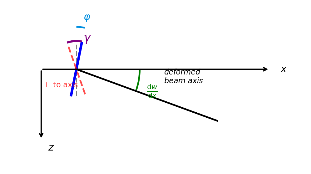
The slope of the deformed beam axis is \(\mathrm{d}w/\mathrm{d}x\). This slope can be decomposed into two contributions: A rotation\(\varphi\), which is the rigid body rotation of the cross-section (positive counterclockwise), and a shear strain\(\gamma\), the angular distortion due to shear deformation.
With \(z\) pointing downward and \(\varphi\) positive counterclockwise, a positive slope \(\mathrm{d}w/\mathrm{d}x\) (beam deflecting further down as \(x\) increases) corresponds to a clockwise rotation, which is negative\(\varphi\). Therefore: \[\frac{\mathrm{d}w}{\mathrm{d}x} = \gamma-\varphi\]
Rearranging, the shear strain\(\gamma\) measures the angular deviation between the cross-section orientation and the beam axis slope: \[\gamma = \frac{\mathrm{d}w}{\mathrm{d}x} + \varphi\]
Figure 3: Shear strain \(\gamma\) as the sum of the slope of the beam axis \(\mathrm{d}w/\mathrm{d}x\) and the rotation of the cross-section \(\varphi\).
If the cross-section remains perpendicular to the deformed beam axis (as in Bernoulli beam theory), then \(\varphi = -\mathrm{d}w/\mathrm{d}x\) and \(\gamma = 0\). A non-zero shear strain indicates that the cross-section is not perpendicular to the beam axis.
Curvature
The curvature\(\chi\) measures the rate of change of rotation along the beam: \[\chi = \frac{\mathrm{d}\varphi}{\mathrm{d}x}\]
Curvature quantifies how much the beam bends per unit length. A positive curvature corresponds to the beam curving such that the center of curvature is below the beam (concave downward in the z-down convention).
NoteSummary of kinematic relations
The kinematic quantities and their relationships are:
Quantity
Symbol
Definition
Physical meaning
Axial displacement
\(u\)
—
Motion along beam axis
Deflection
\(w\)
—
Motion perpendicular to beam
Rotation
\(\varphi\)
—
Rotation of cross-section
Axial strain
\(\varepsilon\)
\(\mathrm{d}u/\mathrm{d}x\)
Stretching of beam axis
Shear strain
\(\gamma\)
\(\mathrm{d}w/\mathrm{d}x + \varphi\)
Angular distortion
Curvature
\(\chi\)
\(\mathrm{d}\varphi/\mathrm{d}x\)
Bending per unit length
Constitutive relations
The strain measures \(\varepsilon\), \(\gamma\), and \(\chi\) describe the local deformation of the beam, but they do not tell us anything about the forces required to produce these deformations. To close the system of equations, we need constitutive relations that connect the kinematic quantities to the internal forces. These relations depend on the material properties and encode how stiff the beam is against different types of deformation.
For a linear elastic beam, the constitutive relations take a particularly simple form: each internal force is proportional to its conjugate strain measure. The normal force \(N\) is proportional to the axial strain, \[N = EA\,\varepsilon,\] where \(E\) is Young’s modulus and \(A\) is the cross-sectional area. The product \(EA\) is called the axial stiffness and determines how much force is needed to stretch the beam by a given amount. A beam with a larger cross-section or made from a stiffer material requires more force to achieve the same axial strain.
Similarly, the shear force \(Q\) is proportional to the shear strain, \[Q = GA\,\gamma,\] where \(G\) is the shear modulus. The product \(GA\) is called the shear stiffness. In practice, a correction factor \(\kappa\) (the Timoshenko shear coefficient) is often introduced to account for the non-uniform distribution of shear stress across the cross-section, giving \(Q = \kappa GA\,\gamma\). For a rectangular cross-section, \(\kappa \approx 5/6\).
Finally, the bending moment \(M\) is proportional to the curvature, \[M = EI\,\chi,\] where \(I\) is the second moment of area (moment of inertia) of the cross-section about the neutral axis. The product \(EI\) is called the flexural rigidity or bending stiffness. This quantity plays a central role in beam theory: it determines how much moment is required to bend the beam by a given amount. The second moment of area \(I\) depends on the shape of the cross-section and how the material is distributed relative to the neutral axis. Moving material away from the neutral axis (as in an I-beam) dramatically increases \(I\) and hence the bending stiffness.
NoteSummary of constitutive relations
The three constitutive relations for a linear elastic beam are:
These relate internal forces (from equilibrium) to kinematic quantities (from geometry).
The Bernoulli hypothesis
So far, we have kept the rotation \(\varphi\) as an independent kinematic variable. This general formulation leads to Timoshenko beam theory, which accounts for shear deformation and is necessary for thick beams or beams made of materials with low shear stiffness. However, for most engineering applications involving slender beams, shear deformation is small compared to bending deformation, and we can make a powerful simplifying assumption.
The Bernoulli hypothesis (also called the Euler-Bernoulli or Navier-Bernoulli assumption) states:
“Plane cross-sections remain plane and perpendicular to the deformed beam axis.”
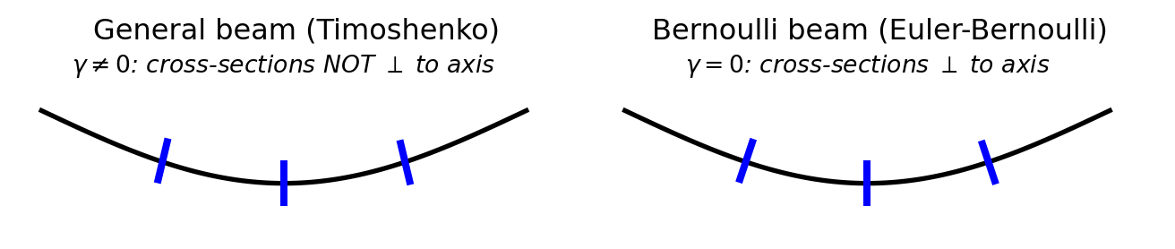
This seemingly simple statement has profound consequences. It says that when a beam bends, each cross-section rotates as a rigid body and always stays at right angles to the curved beam axis. There is no “shearing” of the cross-section relative to the axis—the cross-section simply follows the slope of the beam. Figure 4 illustrates this difference.
Code
import numpy as npimport matplotlib.pyplot as pltfrom matplotlib.patches import Rectangle, FancyArrowPatchfig, (ax1, ax2) = plt.subplots(1, 2, figsize=(7, 3))# Colorsbeam_color ='#cccccc'arrow_color ='#008fe0'# Left panel: General case (with shear)ax1.set_title('General beam (Timoshenko)', fontsize=12)# Draw curved beam axis (z points down, so deflection goes down in plot)x = np.linspace(0, 1, 100)w =-0.15* np.sin(np.pi * x) # negative for z-down conventionax1.plot(x, w, 'k-', linewidth=2, label='beam axis')# Draw cross-sections at various pointsfor x_pos in [0.25, 0.5, 0.75]: idx =int(x_pos *99)# Slope of beam axis in plot coordinates dw_dx_plot =-0.15* np.pi * np.cos(np.pi * x_pos)# Cross-section rotation (different from slope - shear deformation) phi = dw_dx_plot *0.7# not perpendicular cs_length =0.08 dx =-cs_length/2* np.sin(phi) dz = cs_length/2* np.cos(phi) ax1.plot([x_pos - dx, x_pos + dx], [w[idx] - dz, w[idx] + dz], 'b-', linewidth=3)ax1.text(0.5, 0.08, r'$\gamma \neq 0$: cross-sections NOT $\perp$ to axis', fontsize=10, ha='center', style='italic')ax1.set_xlim(-0.05, 1.1)ax1.set_ylim(-0.25, 0.12)ax1.set_aspect('equal')ax1.axis('off')# Right panel: Bernoulli case (no shear)ax2.set_title('Bernoulli beam (Euler-Bernoulli)', fontsize=12)# Draw curved beam axisax2.plot(x, w, 'k-', linewidth=2, label='beam axis')# Draw cross-sections perpendicular to beam axisfor x_pos in [0.25, 0.5, 0.75]: idx =int(x_pos *99)# Slope of beam axis in plot coordinates dw_dx_plot =-0.15* np.pi * np.cos(np.pi * x_pos)# Cross-section rotation equals slope (perpendicular to axis) phi = np.arctan(dw_dx_plot) cs_length =0.08 dx =-cs_length/2* np.sin(phi) dz = cs_length/2* np.cos(phi) ax2.plot([x_pos - dx, x_pos + dx], [w[idx] - dz, w[idx] + dz], 'b-', linewidth=3)ax2.text(0.5, 0.08, r'$\gamma = 0$: cross-sections $\perp$ to axis', fontsize=10, ha='center', style='italic')ax2.set_xlim(-0.05, 1.1)ax2.set_ylim(-0.25, 0.12)ax2.set_aspect('equal')ax2.axis('off')plt.tight_layout()plt.show()
Figure 4: The Bernoulli hypothesis: cross-sections remain perpendicular to the deformed beam axis. This means the rotation \(\varphi\) equals the slope \(\mathrm{d}w/\mathrm{d}x\).
Mathematically, the Bernoulli hypothesis constrains the cross-section rotation to equal the negative of the slope of the beam axis: \[\varphi = -\frac{\mathrm{d}w}{\mathrm{d}x}\] The negative sign arises because with our conventions (\(z\) pointing downward, \(\varphi\) positive counterclockwise), a positive slope \(\mathrm{d}w/\mathrm{d}x\) corresponds to a clockwise rotation, which is negative \(\varphi\).
This constraint has an immediate and important consequence: the shear strain vanishes. Substituting the Bernoulli hypothesis into the shear strain definition gives \[\gamma = \frac{\mathrm{d}w}{\mathrm{d}x} + \varphi = \frac{\mathrm{d}w}{\mathrm{d}x} - \frac{\mathrm{d}w}{\mathrm{d}x} = 0.\] This is the mathematical expression of “perpendicular to the axis”—no shear strain means the cross-section does not tilt relative to the beam axis.
With \(\varphi\) no longer independent, the curvature becomes a function of the deflection alone: \[\chi = \frac{\mathrm{d}\varphi}{\mathrm{d}x} = -\frac{\mathrm{d}^2 w}{\mathrm{d}x^2}.\] This is a crucial simplification: instead of two independent kinematic variables (\(w\) and \(\varphi\)), we now have only one (\(w\)). The entire bending behavior of the beam is captured by a single function—the deflection \(w(x)\).
The Bernoulli hypothesis is an excellent approximation when the beam is slender (its length \(L\) is much larger than its cross-sectional dimensions), when shear deformation is negligible compared to bending deformation, and when the material is homogeneous and isotropic. For short, deep beams or sandwich structures with soft cores, the Timoshenko theory (which retains \(\gamma \neq 0\)) provides more accurate results. As a rule of thumb, Bernoulli beam theory is accurate when the length-to-depth ratio exceeds about 10.
Euler-Bernoulli beam equations
Combining the Bernoulli hypothesis with the constitutive relation for bending:
This is the Euler-Bernoulli beam equation, the fundamental differential equation governing beam deflection.
NoteSign convention
The sign in the Euler-Bernoulli equation depends on the sign conventions used for \(q\), \(Q\), \(M\), and \(w\). With our conventions (positive \(w\) and \(q\) in the positive \(z\)-direction, i.e., downward), we have \(EI\,w'''' = q\). Some textbooks use opposite conventions, resulting in \(EI\,w'''' = -q\).
Boundary conditions
The fourth-order differential equation requires four boundary conditions. These depend on the support type:
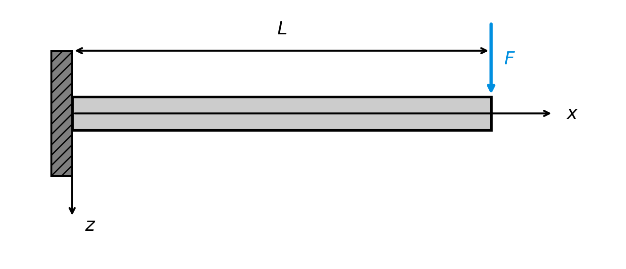
Consider a cantilever beam of length \(L\), fixed at \(x=0\), with a downward point load \(F\) at the free end \(x=L\).
Code
import numpy as npimport matplotlib.pyplot as pltfrom matplotlib.patches import Rectanglefig, ax = plt.subplots(figsize=(7, 3))# Colorsbeam_color ='#cccccc'support_color ='#7f7f7f'load_color ='#008fe0'L =1.0beam_height =0.08# Draw the beambeam = Rectangle((0, -beam_height/2), L, beam_height, facecolor=beam_color, edgecolor='black', linewidth=2)ax.add_patch(beam)# Draw the fixed supportwall_width =0.05wall_height =0.3wall = Rectangle((-wall_width, -wall_height/2), wall_width, wall_height, facecolor=support_color, edgecolor='black', linewidth=1.5, hatch='///')ax.add_patch(wall)# Draw point load arrow (pointing down = positive z direction, from top of beam)arrow_length =0.18ax.annotate('', xy=(L, beam_height/2), xytext=(L, beam_height/2+ arrow_length), arrowprops=dict(arrowstyle='->', color=load_color, lw=2.5))ax.text(L +0.03, beam_height/2+ arrow_length/2, r'$F$', fontsize=14, ha='left', va='center', color=load_color)# Dimension line for Ldim_y =0.15ax.annotate('', xy=(0, dim_y), xytext=(L, dim_y), arrowprops=dict(arrowstyle='<->', color='black', lw=1.5))ax.text(L/2, dim_y +0.04, r'$L$', fontsize=14, ha='center')# Coordinate axesax.annotate('', xy=(1.15, 0), xytext=(0, 0), arrowprops=dict(arrowstyle='->', color='black', lw=1.5))ax.text(1.18, 0, r'$x$', fontsize=14, va='center')ax.annotate('', xy=(0, -0.25), xytext=(0, 0), arrowprops=dict(arrowstyle='->', color='black', lw=1.5))ax.text(0.03, -0.28, r'$z$', fontsize=14, ha='left')ax.set_xlim(-0.15, 1.3)ax.set_ylim(-0.35, 0.25)ax.set_aspect('equal')ax.axis('off')plt.tight_layout()plt.show()
Figure 5: Cantilever beam with point load \(F\) at the free end.
Our goal is to find the deflection \(w(x)\) of the beam. We will solve the Euler-Bernoulli beam equation with appropriate boundary conditions.
For \(0 < x < L\), there is no distributed load (the load is concentrated at the end), so \(q(x) = 0\). The Euler-Bernoulli equation becomes: \[EI\,\frac{\mathrm{d}^4 w}{\mathrm{d}x^4} = 0\]
To solve this fourth-order ordinary differential equation, we need to integrate four times. Each integration introduces one constant of integration, so we expect four unknown constants in our general solution. Integrating the equation \(w'''' = 0\) once gives \(w''' = C_4\) (a constant). Integrating again gives \(w'' = C_4 x + C_3\). Continuing: \[w' = \frac{C_4}{2}x^2 + C_3 x + C_2\]\[w = \frac{C_4}{6}x^3 + \frac{C_3}{2}x^2 + C_2 x + C_1\]
It is conventional to redefine the constants to absorb the numerical factors. Writing the general solution as: \[w(x) = C_1 + C_2 x + C_3 x^2 + C_4 x^3\]
we see that the deflection is a cubic polynomial in \(x\). The four constants \(C_1, C_2, C_3, C_4\) must be determined from boundary conditions.
The fourth-order equation requires exactly four boundary conditions—two at each end of the beam. At the fixed end (\(x=0\)): the beam cannot move vertically, so \(w(0) = 0\), and the beam cannot rotate (the slope is zero), so \(w'(0) = 0\). At the free end (\(x=L\)): there is no bending moment, so \(M(L) = 0\), and a point load \(F\) acts downward, which must equal the shear force, so \(Q(L) = F\).
To use the last two conditions, we need to express \(M\) and \(Q\) in terms of \(w\). From the Euler-Bernoulli theory: \[M = -EI\,w'' \quad \text{and} \quad Q = -EI\,w'''\]
Therefore, the boundary conditions at the free end become: \[w''(L) = 0 \quad \text{and} \quad -EI\,w'''(L) = F\]
Now we apply each boundary condition to determine the constants. From \(w(0) = 0\), we substitute \(x = 0\) into \(w(x) = C_1 + C_2 x + C_3 x^2 + C_4 x^3\): \[w(0) = C_1 + 0 + 0 + 0 = C_1 = 0\]
From \(w'(0) = 0\), we first differentiate \(w(x)\) to get \(w'(x) = C_2 + 2C_3 x + 3C_4 x^2\). Then: \[w'(0) = C_2 + 0 + 0 = C_2 = 0\]
From \(M(L) = -EI\,w''(L) = 0\), we differentiate again to get \(w''(x) = 2C_3 + 6C_4 x\). The condition \(w''(L) = 0\) gives: \[2C_3 + 6C_4 L = 0\]
Solving for \(C_3\): \[C_3 = -3C_4 L\]
From \(Q(L) = -EI\,w'''(L) = F\), we differentiate once more to get \(w'''(x) = 6C_4\). The condition becomes: \[-EI \cdot 6C_4 = F\]
Solving for \(C_4\): \[C_4 = -\frac{F}{6EI}\]
Now we can find \(C_3\) using the relation from the moment condition: \[C_3 = -3C_4 L = -3 \cdot \left(-\frac{F}{6EI}\right) \cdot L = \frac{FL}{2EI}\]
Substituting the constants back into the general solution: \[w(x) = 0 + 0 \cdot x + \frac{FL}{2EI} x^2 + \left(-\frac{F}{6EI}\right) x^3\]
The maximum deflection occurs at the free end, \(x = L\): \[w_{\max} = w(L) = \frac{FL^2}{6EI}(3L - L) = \frac{FL^2}{6EI} \cdot 2L = \frac{FL^3}{3EI}\]
The deflection is positive (downward, since \(z\) points down), which is correct for a downward load. The deflection increases with force \(F\) and length \(L\), and decreases with bending stiffness \(EI\)—all as expected. The cubic dependence on \(L\) explains why long cantilevers deflect much more than short ones.
NoteChapter Summary
This chapter established the kinematic framework for beam analysis: