After completing this chapter, you should be able to:
Construct free body diagrams to identify internal forces (\(N\), \(Q\), \(M\)) at hypothetical cuts
Derive the differential relationships \(q = -dQ/dx\) and \(Q = dM/dx\) from equilibrium
Integrate distributed loads with boundary conditions to sketch shear force and bending moment diagrams
Free body diagrams
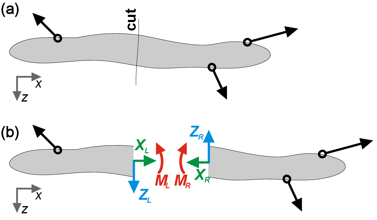
Free body diagrams provide a way to compute forces acting inside the body (internal force variables). By definition, an internal force variable is the resultant of all internal forces in a solid body at a hypothetical cut through the body (Figure 1). If we imagine cutting the body in equilibrium along some line, we technically create two fragments that are no longer in equilibrium. Therefore we need to introduce additional forces on the cut to restore the equilibrium and balance the forces. For a 2D system we can distinguish three resultants on the cut: normal force \(N\) (perpendicular to cut), shear force \(Q\) (parallel to the plane of cut) and bending moment \(M\) (perpendicular to the 2D area of force system). Together with reactions, internal force variables can be determined using a free body diagram.
Figure 1: Internal forces at a hypothetical cut through the body. Note that forces and moment on left and right sides of the cut compensate each other to maintain equilibrium.
By hypothetically splitting the beam into two fragments, we add six internal force variables on the cut (three for left and three for right) that balance both fragments. To keep the whole body in equilibrium after ”gluing” these two fragments back, the internal force variables on the left and right should have the same amplitude and opposite directions. Therefore, by cutting the beam, we increase the number of bodies to \(n=2\), however, we also add three internal constraints, therefore keeping \(D\) constant.
Note
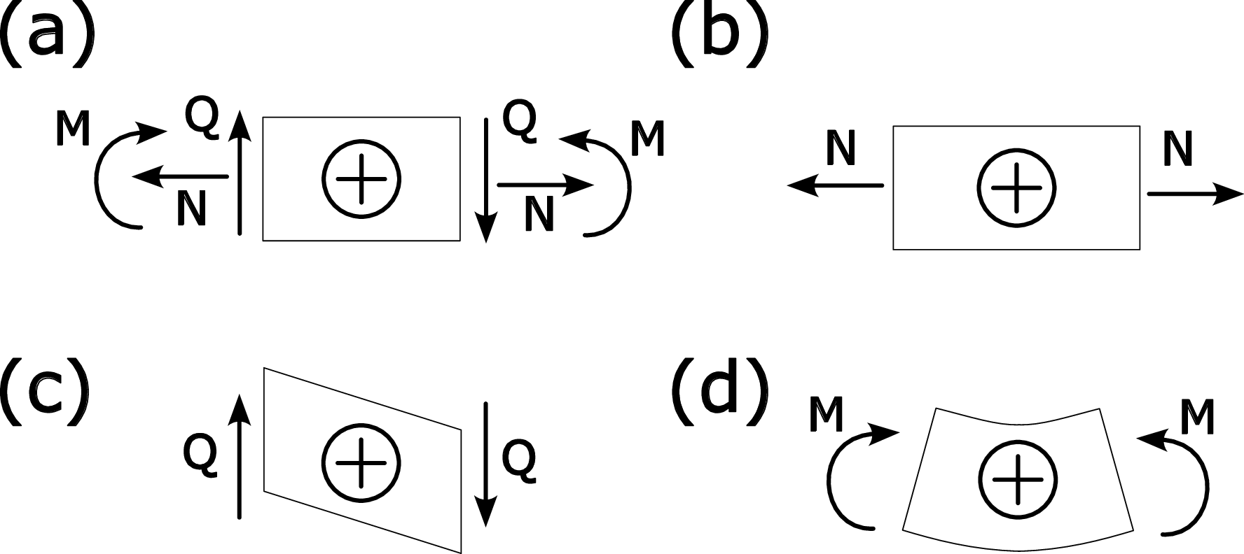
To correctly operate with internal force variables, we need to agree on non-ambiguous sign conventions (Figure 2). We will obey the following rules
Internal forces are positive if the directions on left-hand side and right-hand side of the beam are according to Figure (a), and negative otherwise;
Normal forces are positive if they elongate the beam (b);
Shear forces are positive if the cross-section of the beam slides downward (c);
Bending moments are positive if the bottom of the beam is in extension and the top in compression (d).
Figure 2: (a) Sign conventions for normal force \(N\), shear force \(Q\) and bending moment \(M\). Deformations caused by (b) normal force, (c) shear force and (d) bending moment.
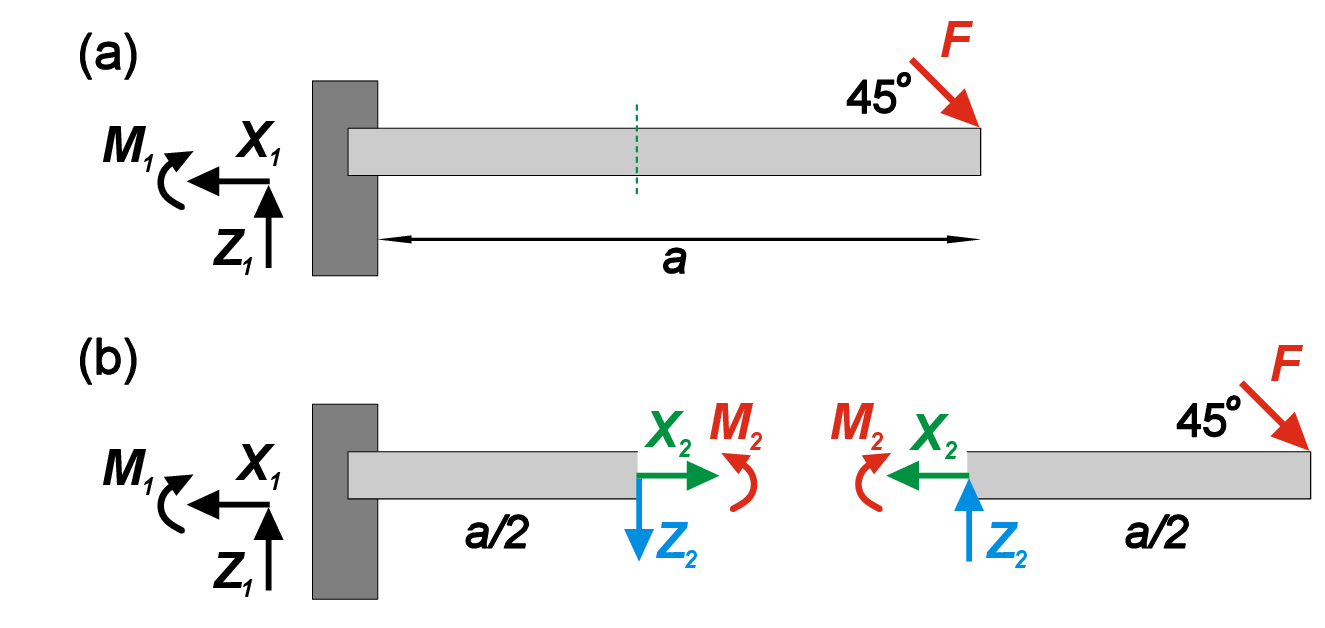
For illustration, let’s consider an example of a beam with length \(a\), that is fixed on the left end and subjected to an inclined point load \(F\) on the right end (Figure 3). We search for the reaction forces as well as internal forces in the middle point of the beam. Simply balancing forces and moments we get \[\begin{aligned} X_1&=F/\sqrt{2} \\ Z_1&=F/\sqrt{2} \\ M_1&=-Fa/\sqrt{2} \end{aligned}\] To find the internal forces and moments at the middle of the beam, we need to cut the beam into two fragments, introduce two reaction forces \(X_2\) and \(Z_2\) and one reaction moment \(M_2\) to preserve equilibrium. Finally, by balancing the forces for both fragments we get \[\begin{aligned} X_2&=F/\sqrt{2} \\ Z_2&=F/\sqrt{2} \\ M_2&=-\frac {Fa}{2\sqrt{2}} \end{aligned} \tag{1}\]
Figure 3: Reaction forces and moments in the beam fixed on the left side and subjected to inclined point load on the right.
Internal force variables
In the previous section, we considered internal forces appearing on the hypothetical cuts. Here we continue discussing internal force variables but with a focus on describing them as a continuous function of the position along the body. From the previous example (Figure 3), we know how to find the internal forces in the middle of the beam (Eq. 3.2). However, we can also perform the same procedure for any other section of the beam. Therefore, it makes sense to consider the reaction forces and moments as functions of the coordinate along the beam length (Fig. 3.3).
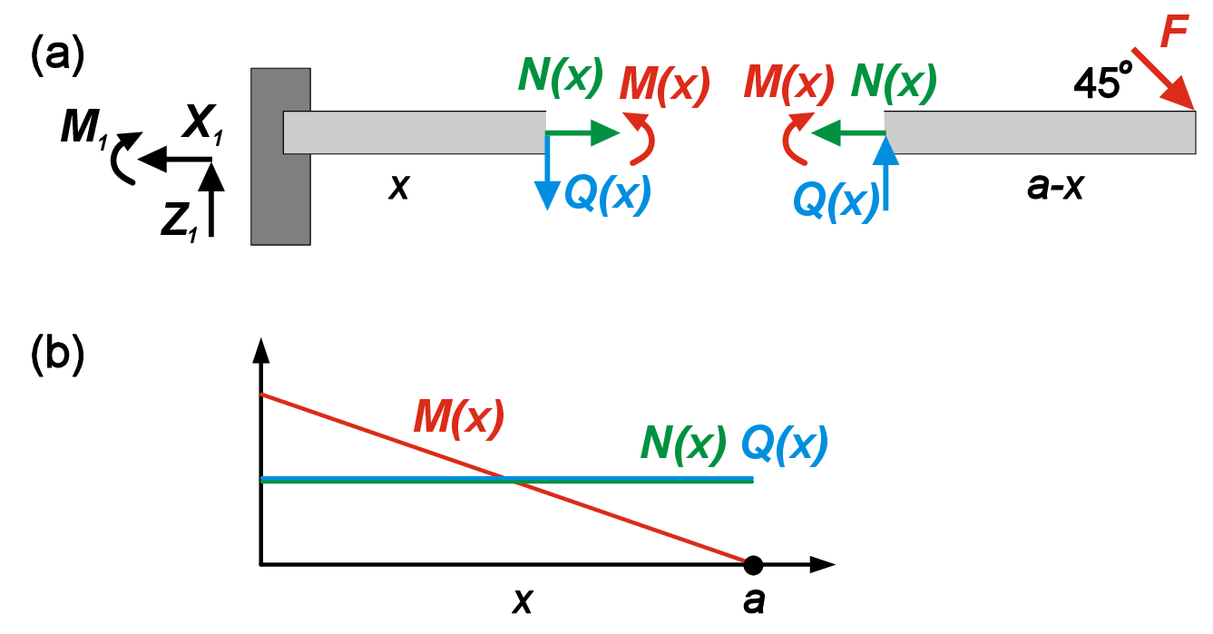
Figure 4: (a) Free body diagram for a beam with intermediate cut. (b) Internal forces and moments diagrams as functions of coordinate \(x\).
Let us consider a cut located at the distance \(x\) from the left hinge/wall (Figure 4). By balancing forces and moments acting on the left and right fragments, it is easy to show that \[\begin{aligned} N(x)&=F/\sqrt{2} \\ Q(x)&=F/\sqrt{2} \\ M(x)&=-\frac {F(a-x)}{\sqrt{2}} \end{aligned} \tag{2}\] Therefore, both longitudinal and shear forces are constant functions of the coordinate \(x\), while moment linearly decreases with an increase in \(x\).
Distributed loads
Prior to this moment, we have considered only idealized point forces. Now we will consider loads distributed along the region of the body (line loads). We will learn how to search for internal forces without exact knowledge of the reaction forces and move towards governing equation of continuum mechanics in the next chapter.
Note
In our next derivations, we will heavily rely on a very useful mathematical concept of Taylor expansion of the function. If we have arbitrary function \(f(x)\), then we can try to approximate it in the vicinity of point \(x_0\) using a polynomial function. So we can find the approximate value of \(f(x+\Delta x)\) just knowing the properties of the function in the point \(x_0\). We will skip the strict mathematical discussion of the necessary conditions and restrictions on function \(f\) and value of \(\Delta x\), and just claim that for a small enough \(\Delta x\) and well-behaved function \(f\), the Taylor expansion provides a good approximation of \(f\). For example, the second order approximation of \(f(x+\Delta x)\) can be expressed as \[\begin{equation} f(x_0+\Delta x)=f(x_0)+\Delta x f'(x_0)+ \frac {1}{2}\Delta x^2 f''(x_0)+O(\Delta x^3) \end{equation}\]In shorter form the general Taylor expansion can be written as \[\begin{equation} f(x_0+\Delta x)=\sum _{i=0}^{\infty }\frac {1}{n!}f^{(i)}(x_0)\Delta x^i \end{equation}\]Note, that \(f^{(i)}\) means \(i-\)th derivative of the function, while \(\Delta x\) is a regular power. In the following, we will use the expression \(\mathrm{d}x\) for (very) small \(\Delta x\), small enough that we can omit all terms \((\mathrm{d}x)^2\) and higher order. The increment \(\mathrm{d}x\) is sometime called an infinitesimal increment.
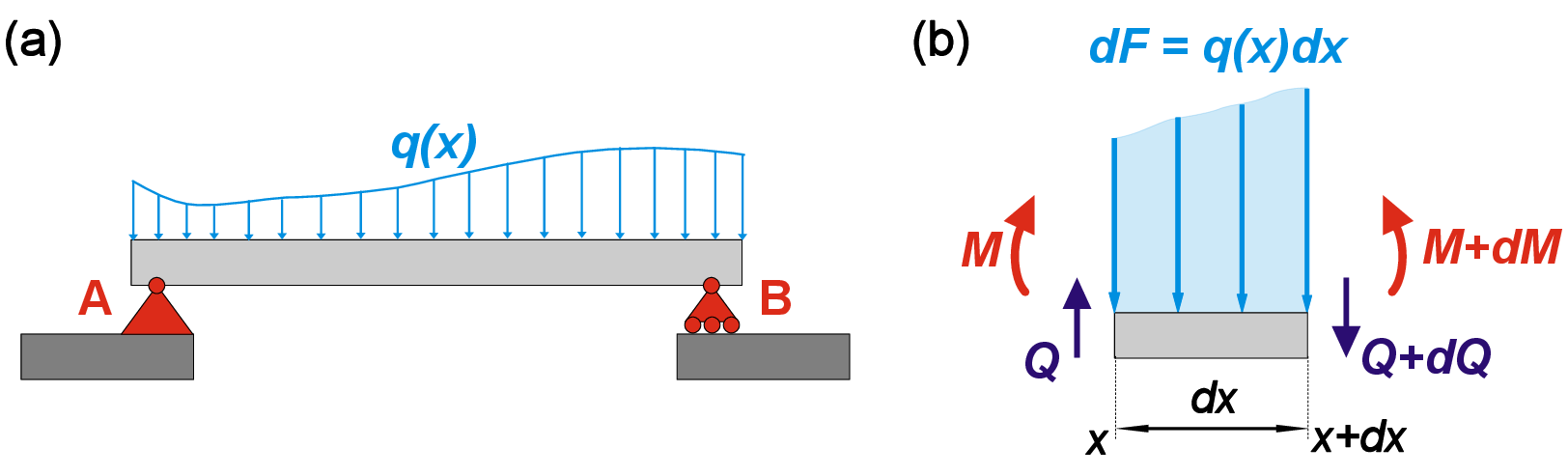
Figure 5: (a) A beam subjected to distributed load. (b) Infinitesimal fragment of beam and corresponding forces.
Let us consider a straight beam subjected to line load that can be expressed as a function of the coordinate \(q(x)\) (Figure 5). We select a very small (infinitesimal) beam element of length \(\mathrm{d}x\) stretching from coordinate \(x\) to \(x+\mathrm{d}x\). Note that here we use \(\mathrm{d}x\) instead of \(\Delta x\) to emphasize the infinitesimal length of this piece. Due to that \(\mathrm{d}x<<(\mathrm{d}x)^2\), and we can use the first order Taylor expansion to find the change in total applied force between left and right ends of the selected beam as \(\mathrm{d}F=q(x)\mathrm{d}x\). Let us now write equilibrium equation for the small piece, taking into account that we can express the shear force and moment on the right side as \(Q(x+\mathrm{d}x)=Q+\mathrm{d}Q\) and \(M(x+\mathrm{d}x)=M+\mathrm{d}M\), respectively, yielding \[Q(x)+\mathrm{d}Q=Q(x)-q(x)\mathrm{d}x.\] We also can write Taylor expansion of \(Q(x)\) at \(x\) as \[Q(x)+\mathrm{d}Q=Q(x)+\frac {\mathrm{d}Q}{\mathrm{d}x}\mathrm{d}x+\ldots\] By comparing coefficients in these two equations, we conclude that \[q(x)=-\frac {\mathrm{d}Q}{\mathrm{d}x} \tag{3}\] This equation establishes the relation between line load and internal shear force in the body. To balance moments, we write \[M(x)+\mathrm{d}M=M(x)+Q(x)\mathrm{d}x.\] Similar to force, we can obtain the first order Taylor expansion and get \[Q(x)=\frac {\mathrm{d}M}{\mathrm{d}x}\]
Governing equations
The governing equations for static equilibrium of a beam are therefore \[\boxed{q(x)=-\frac {\mathrm{d}Q}{\mathrm{d}x} \quad\text{and}\quad Q(x)=\frac {\mathrm{d}M}{\mathrm{d}x}}.\] To solve for the internal forces inside a beam, we need to solve this system of differential equations.
A simple solution procedure is separation of variables. This leads to the generic solution \[\begin {aligned} Q(x)&=-\int {q(x)\mathrm{d}x}+C_1 \\ M(x)&=\int {Q(x)\mathrm{d}x}+C_2.\end {aligned} \tag{4}\] Integration constants \(C_1\) and \(C_2\) have to be found from boundary conditions at bearings and intermediate conditions at connections between body parts. Boundary conditions depend on the bearing type. For example, simple hinge implies \(M=0\), and free end provides two boundary conditions \(M=0\) and \(Q=0\) simultaneously. Note that by computing shear force and moment via integration (Equation 4), we do not need to calculate bearing reactions at all. If we recall the different types of hinges, we can notice that each degree of freedom corresponds to additional equality boundary conditions that can be used to find integration constants (Equation 4).
Example: Fixed cantilever
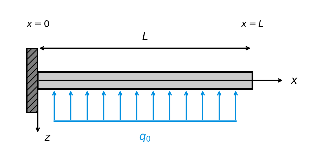
Consider a cantilever beam of length \(L\) fixed at the left end (\(x=0\)) and free at the right end (\(x=L\)), subjected to a constant downward distributed load \(q_0\) (load per unit length).
Figure 6: Cantilever beam with fixed support at the left end and uniform distributed load \(q_0\).
The setup is shown in Figure 6. Our goal is to find how the internal shear force \(Q(x)\) and bending moment \(M(x)\) vary along the length of the beam. We will use the integration method developed above.
The distributed load is constant along the beam: \(q(x) = q_0\). This load acts in the positive \(z\)-direction (downward). Before we can integrate, we need to know what conditions apply at the ends of the beam. At the fixed end (\(x=0\)), the wall provides whatever reaction forces are needed to hold the beam in place—we don’t know \(Q(0)\) or \(M(0)\) in advance, as these are what we’re trying to find. At the free end (\(x=L\)), there is nothing to the right of this point, so no forces or moments can be transmitted. This gives us: \(Q(L) = 0\) and \(M(L) = 0\). The free end boundary conditions are the key to solving this problem.
We start by finding the shear force \(Q(x)\). We use the relationship between distributed load and shear force from Equation 3: \[\frac{\mathrm{d}Q}{\mathrm{d}x} = -q(x) = -q_0\]
To find \(Q(x)\), we integrate both sides with respect to \(x\): \[Q(x) = -\int q_0 \, \mathrm{d}x = -q_0 x + C_1 \tag{5}\]
Here \(C_1\) is an integration constant that we must determine from the boundary condition. We know that at the free end, the shear force must be zero: \(Q(L) = 0\). Substituting \(x = L\) into Equation 5: \[Q(L) = -q_0 L + C_1 = 0\]
Solving for \(C_1\): \[C_1 = q_0 L\]
Now we substitute this back into Equation 5 to get the complete solution: \[Q(x) = -q_0 x + q_0 L = q_0(L - x)\]
At \(x=0\) (fixed end), we get \(Q(0) = q_0 L\). This makes sense: the total distributed load on the beam is \(q_0 \times L\), and all of this load must be transferred to the wall through the shear force at the fixed end. At \(x=L\) (free end), we get \(Q(L) = 0\), which satisfies our boundary condition.
Next we find the bending moment \(M(x)\). We use the relationship between shear force and bending moment from Equation 4: \[\frac{\mathrm{d}M}{\mathrm{d}x} = Q(x) = q_0(L-x)\]
Again, we have an integration constant \(C_2\) to determine. At the free end, the bending moment must be zero: \(M(L) = 0\). Substituting \(x = L\): \[M(L) = q_0\left(L \cdot L - \frac{L^2}{2}\right) + C_2 = q_0\left(L^2 - \frac{L^2}{2}\right) + C_2 = \frac{q_0 L^2}{2} + C_2 = 0\]
This expression can be simplified by factoring. Notice that: \[Lx - \frac{x^2}{2} - \frac{L^2}{2} = -\frac{1}{2}\left(x^2 - 2Lx + L^2\right) = -\frac{1}{2}(L-x)^2\]
Therefore: \[M(x) = -\frac{q_0}{2}(L-x)^2\]
At \(x=L\), we get \(M(L) = 0\) as required. At \(x=0\), we get \(M(0) = -\frac{q_0 L^2}{2}\). The negative sign indicates the moment causes compression at the top of the beam and tension at the bottom, which is the expected behavior for a cantilever with downward loading.
Both shear force and moment diagrams are shown in Figure 7.
Code
import numpy as npimport matplotlib.pyplot as plt# Normalized coordinates (x/L) and normalized load (q0 = 1, L = 1)x = np.linspace(0, 1, 100)# Shear force: Q(x) = q0 * L * (1 - x/L) = q0*L * (1 - xi) where xi = x/L# Normalized: Q / (q0*L)Q_normalized =1- x# Bending moment: M(x) = -q0/2 * (L - x)^2 = -q0*L^2/2 * (1 - x/L)^2# Normalized: M / (q0*L^2)M_normalized =-0.5* (1- x)**2fig, (ax1, ax2) = plt.subplots(2, 1, figsize=(7, 5), sharex=True)# Shear force diagramax1.fill_between(x, 0, Q_normalized, alpha=0.3, color='blue')ax1.plot(x, Q_normalized, 'b-', linewidth=2)ax1.axhline(y=0, color='k', linewidth=0.5)ax1.set_ylabel(r'$Q / (q_0 L)$')ax1.set_title('Shear Force Diagram')ax1.set_ylim(-0.1, 1.2)ax1.grid(True, alpha=0.3)# Bending moment diagramax2.fill_between(x, 0, M_normalized, alpha=0.3, color='red')ax2.plot(x, M_normalized, 'r-', linewidth=2)ax2.axhline(y=0, color='k', linewidth=0.5)ax2.set_xlabel(r'$x / L$')ax2.set_ylabel(r'$M / (q_0 L^2)$')ax2.set_title('Bending Moment Diagram')ax2.set_ylim(-0.6, 0.1)ax2.grid(True, alpha=0.3)plt.tight_layout()plt.show()
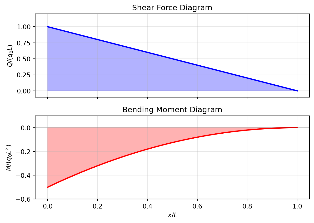
Figure 7: Shear force and bending moment diagrams for a cantilever beam with uniform distributed load \(q_0\).
Key observations:
Shear force: The shear force varies linearly from \(Q(0) = q_0 L\) (fixed end) to \(Q(L) = 0\) (free end)
Bending moment: Parabolic variation with maximum magnitude at the fixed end:
At \(x=0\): \(M(0) = -\frac{q_0 L^2}{2}\) (maximum bending moment, negative per sign convention)
At \(x=L\): \(M(L) = 0\) (free end)
Physical interpretation: The negative moment indicates compression at the top fiber and tension at the bottom fiber, which is the expected deformation pattern for a downward load.
Total load: The total downward load is \(q_0 L\), which equals the reaction shear force at the fixed end, confirming our solution.
NoteChapter Summary
This chapter introduced internal forces in structures:
Free body diagrams: Reveal internal forces by making hypothetical cuts through a structure
Internal force variables: Normal force \(N\) (axial), shear force \(Q\) (transverse), and bending moment \(M\)
Sign conventions: Essential for consistent analysis; positive \(N\) elongates, positive \(M\) creates tension at bottom
Differential relationships: \(q(x) = -dQ/dx\) and \(Q(x) = dM/dx\) connect distributed loads to internal forces
Integration method: Find \(Q(x)\) and \(M(x)\) by integrating load distributions and applying boundary conditions
Boundary conditions: Hinges have \(M=0\); free ends have both \(M=0\) and \(Q=0\)
These internal forces govern how loads are transmitted through structures and will be essential for computing stresses and deformations in later chapters.