Static equilibrium in three dimensions
After completing this chapter, you should be able to:
- Define the Cauchy stress tensor and its components (normal stresses \(\sigma_{ii}\), shear stresses \(\sigma_{ij}\))
- Derive the equilibrium equation \(\nabla \cdot \underline{\sigma} = \vec{f}\) from force balance on a volume element
- Prove that the stress tensor is symmetric (\(\sigma_{ij} = \sigma_{ji}\)) from moment equilibrium
From internal forces to stresses
In previous chapters, we analyzed beams using internal forces: the normal force \(N\), shear force \(Q\), and bending moment \(M\). These quantities are integrals over the cross-section of the beam and provide a simplified description of the mechanical state. However, they hide the detailed distribution of forces within the material. To understand how materials actually carry loads—and when they might fail—we need to look inside the beam and examine the stress distribution.
Consider slicing a beam perpendicular to its axis at some position \(x\). The slice has a cross-sectional area \(A\) with outward normal \(\hat{n}\) pointing in the positive \(x\)-direction. Before we made this imaginary cut, internal forces acted across this surface to hold the two parts of the beam together. These forces are distributed over the entire cross-section, not concentrated at a single point. We have so far ignored these distributed forces; all our beam were slender and we ignored the fact that they have finite thickness.
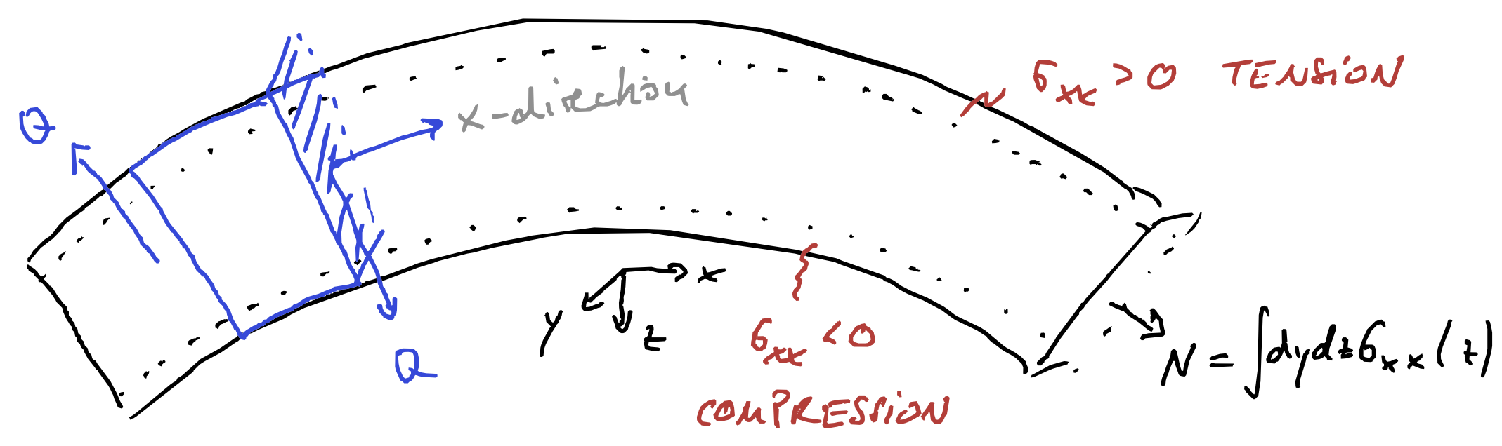
Figure 1 shows a beam with a negative bending moment. Examining a cross-sectional slice, we see that:
- The top of the beam is in tension (material is being pulled apart)
- The bottom is in compression (material is being pushed together)
- Somewhere in between lies the neutral axis whose length stays constant during bending
This distribution of tension and compression cannot be captured by a single force value. We need the concept of stress—force per unit area—to describe how the load is distributed across the section.
Internal forces as stress averages
The internal forces \(N\) and \(Q\) that we computed from equilibrium are actually averages (or more precisely, integrals) of specific stress tensor components over the cross-section:
Normal force is the integral of the normal stress \(\sigma_{xx}\) over the cross-section with area \(A\): \[N(x) = \int_A \mathrm{d}y\mathrm{d}z\,\sigma_{xx}(x,y,z) \tag{1}\]
Shear force is the integral of the shear stress \(\sigma_{xz}\) (or \(\tau_{xz}\)) over the cross-section: \[Q(x) = \int_A \mathrm{d}y\mathrm{d}z\,\sigma_{xz}(x,y,z) \tag{2}\]
Bending moment arises from the moment of the normal stress distribution about the neutral axis, which we assume to be located at \(z=0\): \[M(x) = \int_A \mathrm{d}y\mathrm{d}z\, z \sigma_{xx}(x,y,z) \tag{3}\]
These relationships reveal what internal forces truly represent: they are resultants of stress distributions. A constant normal stress \(\sigma_{xx} = N/A\) across the section would produce the same normal force \(N\), but as Figure 1 shows, the actual stress distribution in bending is far from constant.
The transition from internal forces to stresses is the transition from a 1D beam model to a 2D or 3D continuum description. While internal forces are sufficient for many engineering calculations, understanding stresses is essential for:
- Predicting where a structure will fail (stress concentrations)
- Designing structures with varying cross-sections
- Understanding strain near surfaces, for example to design sensors that measure deformation from surface strain
The stress tensor
In the beam analysis above, we encountered two stress components: the normal stress \(\sigma_{xx}\) (acting perpendicular to the cross-section) and the shear stress \(\sigma_{xz}\) (acting tangent to the cross-section). In a general three-dimensional solid, stresses can act on surfaces oriented in any direction, and the force on each surface can point in any direction. This requires a full tensor to describe.
Consider a small cubic element inside a solid (see e.g. Figure 2), with faces perpendicular to the \(x\), \(y\), and \(z\) axes. On each face, there can be a force per unit area (stress) that has components in all three directions. We use a double-index notation: \(\sigma_{ij}\) denotes the stress component where the first index \(i\) indicates the direction of the force and the second index \(j\) indicates the face on which the force acts (i.e., the face with normal in the \(j\)-direction).
The nine stress components can be organized into a 3×3 matrix called the stress tensor: \[\underline{\sigma} = \begin{pmatrix} \sigma_{xx} & \sigma_{xy} & \sigma_{xz} \\ \sigma_{yx} & \sigma_{yy} & \sigma_{yz} \\ \sigma_{zx} & \sigma_{zy} & \sigma_{zz} \end{pmatrix}\]
The diagonal components \(\sigma_{xx}\), \(\sigma_{yy}\), \(\sigma_{zz}\) are called normal stresses—they act perpendicular to the surface and cause tension (positive) or compression (negative). The off-diagonal components are called shear stresses—they act tangent to the surface and cause angular distortion. The shear stresses are often denoted with the symbol \(\tau\), so \(\tau_{xy} = \sigma_{xy}\), \(\tau_{xz} = \sigma_{xz}\), etc.
As we will show later in this chapter, moment equilibrium requires the stress tensor to be symmetric: \(\sigma_{ij} = \sigma_{ji}\). This means \(\tau_{xy} = \tau_{yx}\), \(\tau_{xz} = \tau_{zx}\), and \(\tau_{yz} = \tau_{zy}\), reducing the number of independent stress components from nine to six.
Static equilibrium
We will treat elasticity exclusively in the limit of small or infinitesimal strains where all equations are linear. The generalization of this “small strain” theory is “finite strain” elasticity which we will not treat in this class. We can make an analogy to the beam: Small strain means we will be ignoring rotations, as in Euler-Bernoulli beam theory. Note that linear elasticity is a classical field theory, this means all quantities typically depend continuously on positions \(\vec{r}\). Those quantities are called fields.
The central quantities of small strain elasticity are the (Cauchy) stress field \(\underline{\sigma }(\vec{r})\) and the displacement field \(\vec{u}(\vec{r})\). Given a material point has moved from position \(\vec{r}\) to \(\vec{r}^{\prime}\), the displacement field is \(\vec{u}(\vec{r})=\vec{r}^{\prime} -\vec{r}\). It therefore describes by how much a volume element in our deformed material has moved (or displaced) because of the deformation and is therefore the generalization of the fields \(u(x)\) and \(w(x)\) that we used to describe the deformation of beams.
The stress \(\underline{\sigma }\) is a tensor that transforms an area (vector) \(\vec{A}\) into a force vector \(\vec{F}\), \[\vec{F}=\underline{\sigma }\cdot \vec{A} \tag{4}\] Note that the area here is a vectorial quantity; the direction of this area vector points outwards on that area, i.e. \(\vec{A}=A \hat{n}\) where \(\hat{n}\) is the normal vector on the respective area.
In three-dimensions, the stress tensor is represented by a \(3\times 3\) matrix. A tensor describes a linear relationship between two quantities; the stress tensor describes the relationship between area of a virtual plane in our solid and the force acting on it, Equation 4. The fact that both force and normal vector of the area are represented in a certain coordinate system implies certain properties of the tensors, in particular for the transformation of the elements of the tensor under rotation of this coordinate system. We will discuss those in detail in the next chapter. For the remainder of this chapter, we only need property Equation 4 of the stress tensor.
We will now consider the equilibrium of forces inside a solid body. Specifically, we regard a small volume element inside this body. Figure 2 a shows a sketch of some body with a volume element highlighted in red. If side lengths of the element \(\Delta x\), \(\Delta y\) and \(\Delta z\) are small enough, then the forces on opposite sites of the element must balance. We here denote the forces on the faces perpendicular to the \(x\)-direction by \(\vec{X}\), the forces on the \(y\)-faces by \(\vec{Y}\) and the forces on the \(z\)-faces by \(\vec{Z}\) (see Figure 2 b, \(z\)-direction not shown). If we know the areas, we can get the forces from the stress tensor \(\underline{\sigma }\) (that converts areas into forces, see Equation 4, specifically \[\vec{X} = \begin{pmatrix} \sigma_{xx} \Delta y \Delta z \\ \sigma_{yx} \Delta y \Delta z \\ \sigma_{zx} \Delta y \Delta z \end{pmatrix},\quad \vec{Y} = \begin{pmatrix} \sigma_{xy} \Delta x \Delta z \\ \sigma_{yy} \Delta x \Delta z \\ \sigma_{zy} \Delta x \Delta z \end{pmatrix} \quad\mathrm{and}\quad \vec{Z} = \begin{pmatrix} \sigma_{xz} \Delta x \Delta y \\ \sigma_{yz} \Delta x \Delta y \\ \sigma_{zz} \Delta x \Delta y \end{pmatrix}. \tag{5}\] Note that \(\vec{X}\), \(\vec{Y}\), \(\vec{Z}\) and \(\underline{\sigma }\) are fields; they explicitly depend on position \(\vec{r}\) within the body.

For a volume element located at position \(\vec{r}=(x,y,z)\), force equilibrium inside the element can be expressed as \[\begin{split}\vec{X}(x+\Delta x, y, z) - \vec{X}(x, y, z) &+ \vec{Y}(x, y+\Delta y, z) - \vec{Y}(x, y, z) \\ &+ \vec{Z}(x, y, z+\Delta z) - \vec{Z}(x, y, z) = \vec{F}(x,y,z) \end{split} \tag{6}\] where \(\vec{F}(x,y,z)\) is an external force, often called the body force, acting on the volume element. We can insert Equation 5 and divide by the volume of the element \(\Delta x \Delta y \Delta z\) to obtain \[\begin{equation} \begin{split} \frac{\sigma_{xx}(x+\Delta x,y,z)-\sigma_{xx}(x, y, z)}{\Delta x} &+ \frac{\sigma_{xy}(x,y+\Delta y,z)-\sigma_{xy}(x, y, z)}{\Delta y} \\ &+\frac{\sigma_{xz}(x,y,z+\Delta z)-\sigma_{xz}(x, y, z)}{\Delta z} = f_x(x,y,z) \end{split} \end{equation}\]for the \(x\)-component of Equation 6. Here \(f_x=F_x/\Delta x \Delta y \Delta z\) is a volume of body force. In the limit \(\Delta x\to 0\) and \(\Delta y\to 0\) this becomes \[\begin{equation} \frac{\partial \sigma_{xx}}{\partial x} + \frac{\partial \sigma_{xy}}{\partial y} + \frac{\partial \sigma_{xz}}{\partial z} = f_x. \end{equation}\]From the \(y\) and \(z\)-component of Equation 6 we get two more differential equations,
\[\begin{align} \frac{\partial \sigma_{yx}}{\partial x} + \frac{\partial \sigma_{yy}}{\partial y} + \frac{\partial \sigma_{yz}}{\partial z} &= f_y \\ \frac{\partial \sigma_{zx}}{\partial x} + \frac{\partial \sigma_{zy}}{\partial y} + \frac{\partial \sigma_{zz}}{\partial z} &= f_z. \end{align}\] These can be summarized to the compact notation \[\text{div}\, \underline{\sigma } \equiv \nabla \cdot \underline{\sigma } = \vec{f}, \tag{7}\] or in words: The divergence of the stress tensor equals the body force. Equation 7 is the central expression of elastostatics that describes force balance within a solid body.
Differential operators in tensor calculus are often defined by means of the Nabla operator \(\nabla\). In our typical \(3\)-dimensional Euclidean space it reads \[\nabla =\begin{pmatrix}\frac{\partial }{\partial x} \\ \frac{\partial }{\partial y} \\ \frac{\partial }{\partial z}\end{pmatrix}=\hat{x}\frac{\partial }{\partial x} + \hat{y}\frac{\partial }{\partial y} + \hat{z}\frac{\partial }{\partial z},\] where \(\hat{x}\) is the unit vector pointing in the \(x\)-direction. When applied to a second-rank tensor, our divergence operator “acts on the right”, i.e. \[\text{div}\, \underline{\sigma } = \nabla \cdot \underline{\sigma }=\sum_{j=1}^3 \frac{\partial}{\partial r_j}\sigma_{ij,j},\] the derivative is taken with respect to the second index. Here, \(r_j\) is a component of the position vector \(\vec{r}\), i.e. \(r_1=x\), \(r_2=y\) and \(r_3=z\). This is a convention and you may encounter textbooks or publications that use different conventions.
An alternative derivation of force balance invokes the divergence theorem. The divergence theorem is an important result of vector analysis. It converts an integral over a volume \(V\) into an integral over the surface \(S\) of this volume. For a vector field \(\vec{f}(\vec{r})\), the divergence theorem states that \[\int_V \mathrm{d}^3 r\, \nabla \cdot \vec{f}(\vec{r}) = \int_{S} \mathrm{d}^2 r\, \vec{f}(\vec{r}) \cdot \hat{n}(\vec{r}) \tag{8}\] Here, \(\hat{n}(\vec{r})\) is the normal vector pointing outward on the surface \(S\) of the volume \(V\). We can integrate Equation 7 over a volume element inside this body of volume \(V\) and surface area \(S(V)\). Using the divergence theorem (sometimes also called Gauss’ theorem), we obtain \[\int_V \mathrm{d}^3 r\, \nabla \cdot \underline{\sigma } = \int_{S(V)} \mathrm{d}^2 r\,\underline{\sigma } \cdot \vec{e}_S = \int_{S(V)} \mathrm{d}^2 r\,\mathrm{d}\vec{F} = \int_V \mathrm{d}^3 r\,\vec{f} \tag{9}\] where \(\vec{e}_S\) is the normal vector pointing outwards on \(S(V)\). The infinitesimal area vector \(\vec{e}_S \mathrm{d}^2 r\) is hence transformed into an (infinitesimal) force vector \(\mathrm{d}\vec{F} = \underline{\sigma } \cdot \vec{e}_S \mathrm{d}^2 r\) and integrated over. Equation 9 hence contains a sum over all forces acting on the surface of the volume element \(V\), and these forces must sum to the body force. It is nothing else than a statement of force balance for any arbitrarily-chosen volume element \(V\) within the solid body.
Moment equilibrium
Besides equilibrium of forces, we also need to fulfill the equilibrium of moments acting on the volume element. The moment around the \(z\)-axis is given by \[\begin{equation} Y_x \Delta y + X_y \Delta x = 0 \end{equation}\]which immediately implies \(\sigma_{yx}=\sigma_{xy}\). The moment equilibrium around the \(x\)- and \(y\)-axes leads to conditions on the other off-diagonal components of \(\underline{\sigma }\), \(\sigma_{zx}=\sigma_{xz}\) and \(\sigma_{zy}=\sigma_{yz}\). By virtue of moment balance, the stress tensor is a symmetric tensor, \(\sigma_{ij}=\sigma_{ji}\) or \(\underline{\sigma }=\underline{\sigma }^T\).
This chapter introduced the stress tensor and equilibrium equations:
- Stress tensor: The Cauchy stress \(\underline{\sigma}\) transforms area vectors into force vectors: \(\vec{F} = \underline{\sigma} \cdot \vec{A}\)
- Components: Normal stresses (\(\sigma_{xx}\), \(\sigma_{yy}\), \(\sigma_{zz}\)) cause tension/compression; shear stresses (\(\sigma_{xy}\), etc.) cause angular distortion
- Force equilibrium: \(\nabla \cdot \underline{\sigma} = \vec{f}\) states that the divergence of stress equals the body force
- Divergence theorem: Converts volume integrals to surface integrals for force balance
- Moment equilibrium: Requires the stress tensor to be symmetric: \(\sigma_{ij} = \sigma_{ji}\)
- Notation: Vectors use arrows (\(\vec{v}\)), tensors use underlines (\(\underline{\sigma}\))
These equations form the foundation of 3D elastostatics and must be satisfied throughout any deformable body in static equilibrium.