Chapter 10
Nonlinear problems
Context: We have so far considered linear problems. However, we have already encountered the Poisson–Boltzmann equation as an example of a nonlinear partial differential equation. Solving nonlinear partial differential equations introduces two additional levels of difficulty: First, we have to calculate integrals over functions with a polynomial of order higher than two in the basis function. Second, we have to be able to solve a nonlinear system of equations. This chapter introduces numerical quadrature and the Newton-Raphson method as mathematical tools for nonlinear equations.
10.1 Numerical quadrature
The term quadrature is a synonym for integration, but quadrature is often used in contexts where integrals are approximated with numerical methods. The integrals that we have encountered so far were of the form \begin {equation} \left (\frac {\dif ^k N_I^{(e)}}{\dif x^k}, \frac {\dif ^l N_J^{(e)}}{\dif x^l}\right ) = \int _e \dif x\, \frac {\dif ^k N_I^{(e)}}{\dif x^k} \frac {\dif ^l N_J^{(e)}}{\dif x^l} \end {equation} i.e. integrals over combinations of shape functions (or basis functions) and their derivatives. Since we have only worked with linear finite-element basis functions, we needed to integrate constant, linear or quadratic functions, which all are trivial to solve analytically. All the integrals from the previous chapters, in particular the integrals of the Laplace and mass matrices, yielded closed-form expressions. This is in many cases no longer possible with nonlinear PDGLs.
Example: We can use the Debye length to write the nonlinear Poisson-Boltzmann equation as \begin {equation} \tilde {\nabla }^2 \tilde {\Phi } = \sinh \tilde \Phi \label {eq:nondimensionalpb} \end {equation} with the nondimensionalized potential \(\tilde {\Phi } = \varepsilon \tilde {\Phi }/(2\rho _0 \lambda ^2)\) and the nondimensionalized length \(\tilde {x}=x/\lambda \) (or \(\dif /\dif \tilde {x}=\lambda \dif /\dif x\)). In the following, we will work with Eq. \eqref{eq:nondimensionalpb}, but, for the sake of notational simplicity, we will not write the tilde explicitly.
We now consider the one-dimensional version of the nonlinear PB equation on the interval \([0,L]\). The residual is given by \begin {equation} R(x) = \frac {\dif ^2 \Phi }{\dif x^2} - \sinh \Phi . \end {equation} To construct the element matrix, we multiply with a shape function \(N_I(x)\), \begin {equation} \begin {split} (N_I, R) &= \left (N_I, \frac {\dif ^2 \Phi }{\dif x^2} \right ) - (N_I, \sinh \Phi ) \\ &= \left . N_I\frac {\dif \Phi }{\dif x}\right |_0^L - \left (\frac {\dif N_I}{\dif x}, \frac {\dif \Phi }{\dif x}\right ) - (N_I, \sinh \Phi ). \end {split} \end {equation} The function itself on the element is approximated by, \begin {equation} \Phi (x) = a_1 N_1(x) + a_2 N_2(x), \end {equation} yielding \begin {equation} (N_I, R) = -\left (\frac {\dif N_I}{\dif x}, a_1\frac {\dif N_1}{\dif x}+a_2\frac {\dif N_2}{\dif x}\right ) - \left (N_I, \sinh (a_1 N_1+a_2 N_2)\right ). \label {eq:pb-residual} \end {equation} Here, \(a_1\) and \(a_2\) denote the function values at the left and right node of the element. The first term on the right-hand side of Eq. \eqref{eq:pb-residual} can be solved analytically and contains the well-known Laplace matrix. The second term is nonlinear in \(\Phi _N\). The integration is difficult to carry out analytically.
Consider some function \(f(x)\) and the integral \(\int _{-1}^1 \dif x \, f(x)\) over the domain \([-1,1]\). (We restrict ourselves to this domain. An integration over a general interval \([a,b]\) can always be mapped to this domain.) An obvious solution would be to approximate the integral with a sum of rectangles, which is also called a Riemann sum. We write \begin {equation} \int _{-1}^1 \dif x \, f(x) \approx \sum _{n=1}^{N} w^\text {Q}_n f(x^\text {Q}_n). \label {eq:quadrature} \end {equation} Equation \eqref{eq:quadrature} is a quadrature rule. The points \(x_n^\text {Q}\) are called “quadrature points” and the \(w_n^\text {Q}\) are the “quadrature weights”. For the rectangle rule, these weights are exactly the width of the rectangles; other forms of quadrature rules will be discussed below.
Note: The weights of the quadrature rule need to fulfill certain conditions (sometimes also called sum rules). For example, \(\sum _{n=1}^N w^\text {Q}_n = b-a = 2\) because the integral over \(f(x)=1\) must yield the length of the domain. We assume that quadrature points are ordered, i.e. \(x_n^\text {Q} < x_{n+1}^\text {Q}\). Then quadrature point \(x_n^\text {Q}\) must then lie in the \(n\)th interval, \(\sum _{i=1}^{n-1} w_i^\text {Q} < 1 + x_n^\text {Q} < \sum _{i=1}^{n} w_i^\text {Q}\).
We now ask which values of \(x_n^\text {Q}\) and \(w_n^\text {Q}\) would be ideal for a given number of quadrature points \(N\). A good choice for \(N=1\) is certainly \(x_1^\text {Q}=0\) and \(w_1^\text {Q}=2\). This rule leads to the exact solution for linear functions. If we move the quadrature point \(x_1^\text {Q}\) to a different location, only constant functions are integrated exactly.
Example: A linear function \begin {equation} f(x) = A + Bx \end {equation} integrates to \begin {equation} \int _{-1}^1 \dif x\, f(x) = \left [Ax + Bx^2/2\right ]_{-1}^1 = 2A. \end {equation} The quadrature rule with \(x_1^\text {Q}=0\) and \(w_1^\text {Q}=2\) yields \begin {equation} \int _{-1}^1 \dif x\, f(x) = w^\text {Q}_1 f(x^\text {Q}_1) = 2 f(0) = 2 A, \end {equation} which is the exact result.
A quadratic function \begin {equation} f(x) = A + Bx + Cx^2 \end {equation} integrates to \begin {equation} \int _{-1}^1 \dif x\, f(x) = \left [Ax + Bx^2/2 + Cx^3/3\right ]_{-1}^1 = 2A + 2C/3. \end {equation} The quadrature rule yields \begin {equation} \int _{-1}^1 \dif x\, f(x) = w^\text {Q}_1 f(x^\text {Q}_1) = 2 f(0) = 2 A, \end {equation} which is missing the \(2C/3\) term.
With two quadrature points, we should be able to integrate a third-order polynomial exactly. We can determine these points by explicitly demanding the exact integration of polynomials up to the third order with a sum consisting of two terms: \begin {align} \int _{-1}^1 \dif x\, 1 &= 2 = w_1^\text {Q} + w_2^\text {Q} \\ \int _{-1}^1 \dif x\, x &= 0 = w_1^\text {Q} x_1^\text {Q} + w_2^\text {Q} x_2^\text {Q} \\ \int _{-1}^1 \dif x\, x^2 &= 2/3 = w_1^\text {Q} (x_1^\text {Q})^2 + w_2^\text {Q} (x_2^\text {Q})^2 \\ \int _{-1}^1 \dif x\, x^3 &= 0 = w_1^\text {Q} (x_1^\text {Q})^3 + w_2^\text {Q} (x_2^\text {Q})^3 \end {align}
Solving these four equations leads directly to \begin {equation} w_1^\text {Q}=w_2^\text {Q}=1, \quad x_1^\text {Q}=1/\sqrt {3} \quad \text {and}\quad x_2^\text {Q}=-1/\sqrt {3}. \end {equation} For three quadrature points, an identical construction yields \begin {equation} w_1^\text {Q}=w_3^\text {Q}=5/9, \quad w_2^\text {Q}=8/9, \quad x_1^\text {Q}=-\sqrt {3/5}, \quad x_2^\text {Q}=0 \quad \text {and}\quad x_3^\text {Q}=\sqrt {3/5} \end {equation} This type of numerical integration is called Gaussian quadrature.
For integrals over arbitrary intervals \([a,b]\), we have to rescale the quadrature rules. By substituting \(y = (a+b+(b-a)x)/2\), we get \begin {equation} \int _a^b \dif y f(y) = \frac {b-a}{2} \int _{-1}^1 \dif x f(y(x)) \approx \frac {b-a}{2} \sum _{n=0}^{N-1} w_n^\text {Q} f(y(x_n^\text {Q})), \label {eq:scaledquad} \end {equation} where the weights \(w_n^\text {Q}\) and the quadrature points \(x_n^\text {Q}\) are calculated for the interval \([-1,1]\). Quadrature points and weights can often be found in tabulated form, e.g. on Wikipedia.
Note: Gaussian quadrature is also often called Legendre-Gaussian quadrature, since there is a connection between the quadrature points and the roots of the Legendre polynomials.
A simple implementation of Gauss quadrature could look like this:
1def gauss_quad(a, b, f):
2 # Gauss points in the interval [-1, 1] and weights
3 x = np.array([-1/np.sqrt(3), 1/np.sqrt(3)])
4 w = np.array([1, 1])
5 return (b-a)/2 * np.sum(w*f(a + (b-a)*(x+1)/2))
10.1.1 Poisson-Boltzmann equation
Recall the residual of the PB equation, Eq. \eqref{eq:pb-residual}, \begin {equation} (N_I^{(e)}, R) = -\left (\frac {\dif N_I^{(e)}}{\dif x}, a_1^{(e)}\frac {\dif N_1^{(e)}}{\dif x}+a_2^{(e)}\frac {\dif N_2^{(e)}}{\dif x}\right ) - \left (N_I^{(e)}, \sinh \left (a_1^{(e)} N_1^{(e)}+a_2^{(e)} N_2^{(e)}\right )\right ), \end {equation} where \(a_1^{(e)}\) and \(a_2^{(e)}\) are the values at the left and right node of the element \(e\). In the following we will drop the explicit element index \(e\) for brevity and will reintroduce it where necessary. The first term as the well-known Laplace operator with the known (and constant) Laplace matrix \(L_{IJ}=(\dif N_I/\dif x, \dif N_J/\dif x)\). The Laplace matrix is constant because the Laplace operator is linear.
We now approximate the third and nonlinear term \(\left (N_I, \sinh (a_1 N_1+a_2 N_2)\right )\) using Gaussian quadrature, \begin {equation} \begin {split} \left (N_I, \sinh \Phi \right ) &= \int _e\dif x\, N_I(x) \sinh \left (a_1 N_1(x)+a_2 N_2(x)\right ) \\ &= \sum _{i} \frac {\Delta x}{2} w_i^\text {Q} N_I(x_i) \sinh \left (a_1 N_1(x_i)+a_2 N_2(x_i)\right ) \end {split} \end {equation} The sum here runs over the quadrature points \(i\) within element \(e\). Furthermore, \(\Delta x\) is the length of the element; the term \(\Delta x/2\) comes from the rescaling of the quadrature rule, Eq. \eqref{eq:scaledquad}. Furthermore, \(x_i\) is the position of the \(i\)th quadrature point within element \(e\). For a single quadrature point with \(w_0^\text {Q}=2\) and \(N_I(x_0)=1/2\) this yields \begin {equation} \left (N_I, \sinh \Phi \right ) = \frac {\Delta x}{2} \sinh \left (\frac {a_1 +a_2}{2}\right ). \end {equation}
The total residual for basis function \(k\) then becomes the sum over all elements that share node \(k\), in one dimension explicitly \begin {equation} \begin {split} R_k=(\varphi _k, R) =& (N_2^{(k-1)}, R) + (N_1^{(k)}, R) \\ =& L_{21}^{(k-1)}a_{k-1} + L_{22}^{(k-1)}a_k + L_{11}^{(k)}a_k + L_{12}^{(k)}a_{k+1} \\ & + \frac {\Delta x^{(k-1)}}{2} \sinh \left (\frac {a_{k-1} +a_k}{2}\right ) + \frac {\Delta x^{(k)}}{2} \sinh \left (\frac {a_k +a_{k+1}}{2}\right ). \end {split} \end {equation}
We are now looking for the coefficients \(a_n\) for which \(R_k=0\) for all \(k\). This requires an algorithm for finding the roots of a system of nonlinear equations, which we discuss in the next chapter.
10.1.2 Implementation
In practical implementations of nonlinear problems, it is often easier to simply implement numerical quadrature and not use the analytic element matrices. For linear finite elements, the integrals of linear operators are at most quadratic and hence we can exactly integrate them with two quadrature points. We start by implementing the shape functions:
1shape_functions = [
2 lambda zeta: 1 - zeta,
3 lambda zeta: zeta
4]
5
6shape_function_derivatives = [
7 lambda zeta: -np.ones_like(zeta),
8 lambda zeta: np.ones_like(zeta)
9]
The residuals per element, \((N_I, R)\), can then be computed directly from the quadrature rules
1def element_residual(x1, x2, a1, a2):
2 """Residual per element"""
3 width = x2 - x1 # Width/size of the element
4 def f(sf, dsf, x):
5 # sf is shape function N_I
6 # dsf is shape function derivative dN_I/dx
7 r = -dsf(x) * (a1*shape_function_derivatives[0](x) +
8 a2*shape_function_derivatives[1](x))
9 r -= sf(x) * np.sinh(a1*shape_functions[0](x) +
10 a2*shape_functions[1](x))
11 return r
12 retvals = []
13 for sf, dsf in zip(shape_functions,
14 shape_function_derivatives):
15 retvals += [
16 # Integrate over normalized interval [0, 1]
17 width * gauss_quad(0, 1, lambda x: f(sf, dsf, x))
18 ]
19 return retvals
10.2 Newton-Raphson method
The Newton-Raphson method, or just the Newton method, is a method for the iterative solution of a nonlinear equation. For illustration, we will first describe it for scalar-valued functions and then generalize the method for vector-valued functions.
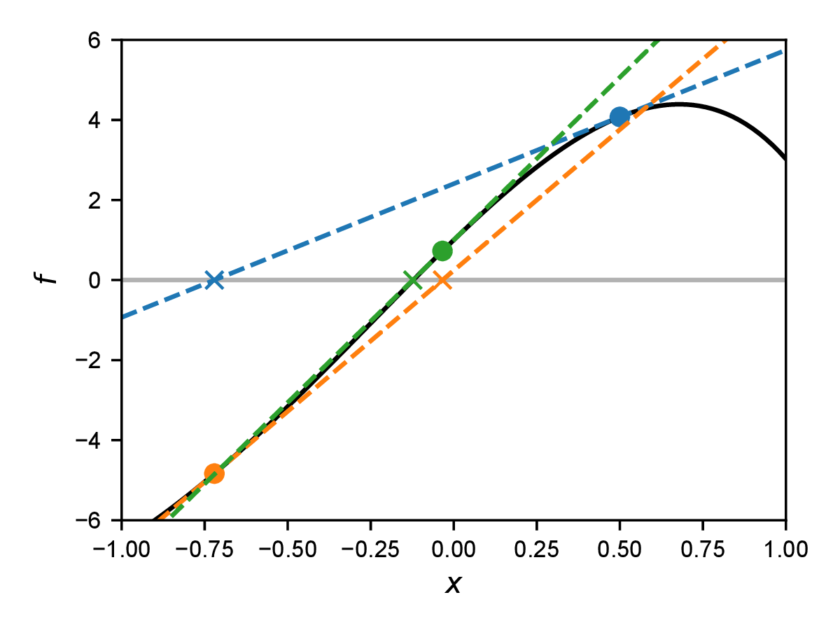
We are looking for a solution of the equation \(f(x)=0\) for an arbitrary function \(f(x)\). Note that generally there can be arbitrary many solution, but the algorithm will only pick one. The idea of the Newton method is to linearize the equation at a point \(x_i\), i.e. to write a Taylor expansion up to first order, and then to solve this linearized system. The Taylor expansion of the equation at \(x_i\) \begin {equation} f(x) \approx f(x_i) + (x - x_i) f'(x_i) = 0 \label {eq:newtonapprox} \end {equation} has the root \(x_{i+1}\) given by \begin {equation} x_{i+1} = x_i - f(x_i) / f'(x_i), \end {equation} where \(f'(x)=\dif f/\dif x\) is the first derivative of the function \(f\). The value \(x_{i+1}\) is now (hopefully) closer to the root \(x_0\) (with \(f(x_0)=0\)) than the value \(x_i\). The idea of the Newton method is to construct a sequence \(x_i\) of linear approximations of the function \(f\) that converges to \(x_0\). We therefore use the root of the linearized form of the equation as the starting point for the next iteration. An example of such an iteration is shown in Fig. 10.1.
The discretization of our nonlinear PDGLs led us to a system of equations \(R_k(\v {a})=0\). We write this here as \(\v {f}(\v {x})=\v {0}\). The Newton method for solving such coupled nonlinear equations works analogously to the scalar case. We first write the Taylor expansion \begin {equation} \v {f}(\v {x}) \approx \v {f}(\v {x}_i) + \t {K}(\v {x}_i)\cdot (\v {x} - \v {x}_i) = 0 \label {eq:newtonapproxmultidim} \end {equation} with the Jacobi matrix \begin {equation} K_{mn}(\v {x})=\frac {\dif f_m(\v {x})}{\dif x_n}. \end {equation} In the context of finite elements, \(\t {K}(\v {x}_i)\) is also often referred to as the tangent matrix or tangent stiffness matrix.
The Newton method can then be written as \begin {equation} \v {x}_{i+1} = \v {x}_i - \t {K}^{-1}(\v {x}_i)\cdot \v {f}(\v {x}_i). \label {eq:newtonmultidim} \end {equation} In the numerical solution of Eq. \eqref{eq:newtonmultidim}, the step \(\Delta \v {x}_i = \v {x}_{i+1} - \v {x}_i\) is usually approximated by solving the linear linear system of equations \(\t {K}(\v {x}_i)\cdot \Delta \v {x}_i = -\v {f}(\v {x}_i)\) and not by using an explicit matrix inversion of \(\t {K}(\v {x}_i)\).
For a purely linear problem, as discussed exclusively in the previous chapters, the tangent matrix \(\t {K}\) is constant and takes on the role of the system matrix. In this case, the Newton method converges in a single step.
10.2.1 Example: Poisson-Boltzmann equation
To use the Newton method, we still need to determine the tangent matrix for the Poisson-Boltzmann equation. To do this, we linearize \(R_k\) in \(a_n\). This yields \begin {equation} K_{IJ}=\frac {\partial (N_I, R)}{\partial a_J} = -L_{IJ} - \sum _{i} \frac {\Delta x}{2} w_i^\text {Q} N_I(x_i) N_J(x_i) \cosh \left (a_1 N_1(x_i)+a_2 N_2(x_i)\right ). \end {equation} The second term has a structure similar to the mass matrix and we write \begin {equation} M_{IJ} = \sum _{i} \frac {\Delta x}{2} w_i^\text {Q} N_I(x_i) N_J(x_i) \cosh \left (a_1 N_1(x_i)+a_2 N_2(x_i)\right ). \label {eq:massmatrixnonlinear} \end {equation} The entire tangent matrix for element \(e\) is therefore \(\t {K}^{(e)}(\v {a})=-\t {L}^{(e)}-\t {M}^{(e)}(\v {a})\), where \(\t {M}^{(e)}(\v {a})\) explicitly depends on the state \(\v {a}\) of the Newton iteration. For a purely linear problem, \(\t {K}^{(e)}\) is the element matrix and does not depend on \(\v {a}\). (Linearization yields \(\cosh x\approx 1\).) The system tangent matrix can be constructed from the element tangent matrix \(K_{IJ}\) using the standard assembly process.
The expression for integration becomes particularly simple with only one Gaussian quadrature point. Then \(w_0^\text {Q}=2\) and \(x_0\) lies exactly in the center of the respective element \(e\), so that \(N_I(x_0)=1/2\). This yields \begin {equation} M_{IJ} = \frac {\Delta x}{4} \cosh \left ( \frac {a_1 + a_2}{2} \right ). \label {eq:PBtangentonequad} \end {equation}