Beispiele

Beispiel 1: Schwach gedämpfter Oszillator

Problemstellung

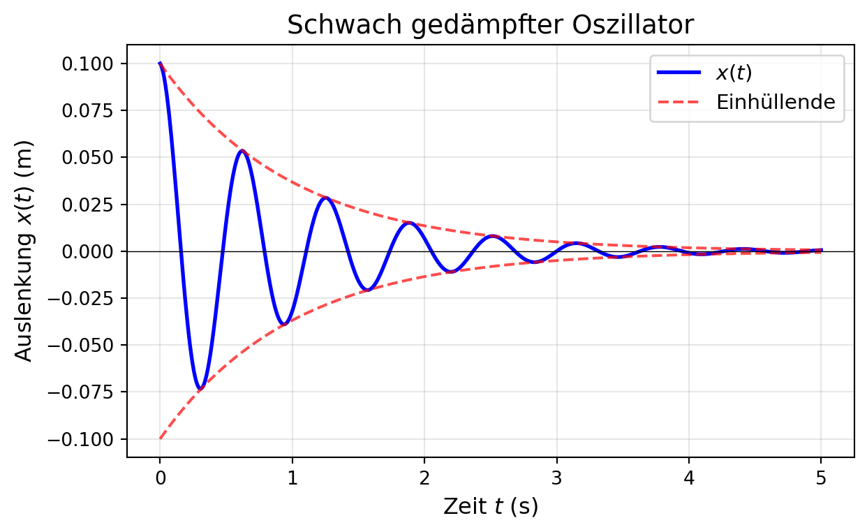
Ein Masse-Feder-System mit \(m = 1\,\text{kg}\), \(k = 100\,\text{N/m}\) und \(c = 2\,\text{Ns/m}\) wird aus der Ruhelage um \(x_0 = 0.1\,\text{m}\) ausgelenkt und dann losgelassen. Bestimmen Sie die Bewegung des Systems.

Lösung

Zunächst berechnen wir die charakteristischen Parameter: \[ \omega_0 = \sqrt{\frac{k}{m}} = \sqrt{\frac{100}{1}} = 10\,\text{rad/s} \]

\[ \gamma = \frac{c}{2m} = \frac{2}{2 \cdot 1} = 1\,\text{s}^{-1} \]

Da \(\gamma = 1 < \omega_0 = 10\), liegt schwache Dämpfung vor. Die gedämpfte Frequenz ist: \[ \omega_d = \sqrt{\omega_0^2 - \gamma^2} = \sqrt{100 - 1} = \sqrt{99} \approx 9.95\,\text{rad/s} \]

Die allgemeine Lösung für schwache Dämpfung lautet: \[ x(t) = A e^{-\gamma t} \cos(\omega_d t + \phi) \]

Mit den Anfangsbedingungen \(x(0) = 0.1\) und \(\dot{x}(0) = 0\) ergibt sich: \[ A = 0.1\,\text{m}, \quad \phi = 0 \]

Die Lösung ist daher: \[ x(t) = 0.1 e^{-t} \cos(9.95t)\,\text{m} \]

import numpy as np
import matplotlib.pyplot as plt

# Parameter
m = 1.0  # kg
k = 100.0  # N/m
c = 2.0  # Ns/m

omega_0 = np.sqrt(k/m)
gamma = c/(2*m)
omega_d = np.sqrt(omega_0**2 - gamma**2)

# Anfangsbedingungen
x0 = 0.1  # m
v0 = 0.0  # m/s

# Zeit
t = np.linspace(0, 5, 1000)

# Lösung
x = x0 * np.exp(-gamma * t) * np.cos(omega_d * t)

# Einhüllende
envelope_upper = x0 * np.exp(-gamma * t)
envelope_lower = -x0 * np.exp(-gamma * t)

plt.figure(figsize=(7, 4))
plt.plot(t, x, 'b-', linewidth=2, label='$x(t)$')
plt.plot(t, envelope_upper, 'r--', linewidth=1.5, alpha=0.7, label='Einhüllende')
plt.plot(t, envelope_lower, 'r--', linewidth=1.5, alpha=0.7)
plt.axhline(y=0, color='k', linestyle='-', linewidth=0.5)
plt.xlabel('Zeit $t$ (s)', fontsize=12)
plt.ylabel('Auslenkung $x(t)$ (m)', fontsize=12)
plt.title('Schwach gedämpfter Oszillator', fontsize=14)
plt.grid(True, alpha=0.3)
plt.legend(fontsize=11)
plt.show()

Abbildung 1: Schwach gedämpfter harmonischer Oszillator

Beispiel 2: Stark gedämpfter Oszillator

Problemstellung

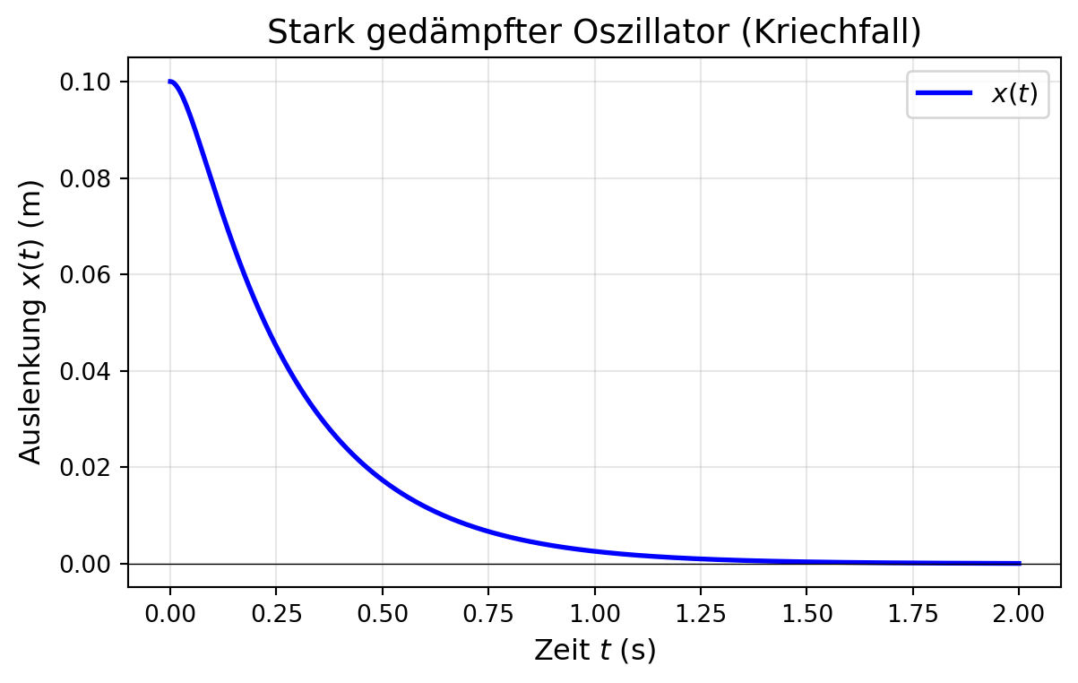
Dasselbe System wie oben, aber mit erhöhter Dämpfung \(c = 30\,\text{Ns/m}\).

Lösung

Die charakteristischen Parameter sind: \[ \omega_0 = 10\,\text{rad/s}, \quad \gamma = \frac{30}{2} = 15\,\text{s}^{-1} \]

Da \(\gamma = 15 > \omega_0 = 10\), liegt starke Dämpfung vor. Die Lösungen der charakteristischen Gleichung sind: \[ \lambda_{1,2} = -\gamma \pm \sqrt{\gamma^2 - \omega_0^2} = -15 \pm \sqrt{225 - 100} = -15 \pm \sqrt{125} \]

\[ \lambda_1 \approx -3.82, \quad \lambda_2 \approx -26.18 \]

Die allgemeine Lösung lautet: \[ x(t) = C_1 e^{\lambda_1 t} + C_2 e^{\lambda_2 t} \]

Mit den Anfangsbedingungen \(x(0) = 0.1\) und \(\dot{x}(0) = 0\) ergibt sich nach Einsetzen: \[ x(t) = 0.117 e^{-3.82t} - 0.017 e^{-26.18t}\,\text{m} \]

import numpy as np
import matplotlib.pyplot as plt

# Parameter für starke Dämpfung
m = 1.0
k = 100.0
c = 30.0

omega_0 = np.sqrt(k/m)
gamma = c/(2*m)

# Charakteristische Werte
lambda1 = -gamma + np.sqrt(gamma**2 - omega_0**2)
lambda2 = -gamma - np.sqrt(gamma**2 - omega_0**2)

# Anfangsbedingungen
x0 = 0.1
v0 = 0.0

# Koeffizienten aus Anfangsbedingungen
C2 = (v0 - lambda1*x0)/(lambda2 - lambda1)
C1 = x0 - C2

# Zeit
t = np.linspace(0, 2, 1000)

# Lösung
x = C1 * np.exp(lambda1 * t) + C2 * np.exp(lambda2 * t)

plt.figure(figsize=(7, 4))
plt.plot(t, x, 'b-', linewidth=2, label='$x(t)$')
plt.axhline(y=0, color='k', linestyle='-', linewidth=0.5)
plt.xlabel('Zeit $t$ (s)', fontsize=12)
plt.ylabel('Auslenkung $x(t)$ (m)', fontsize=12)
plt.title('Stark gedämpfter Oszillator (Kriechfall)', fontsize=14)
plt.grid(True, alpha=0.3)
plt.legend(fontsize=11)
plt.show()

Abbildung 2: Stark gedämpfter harmonischer Oszillator

Beispiel 3: Kritisch gedämpfter Oszillator

Problemstellung

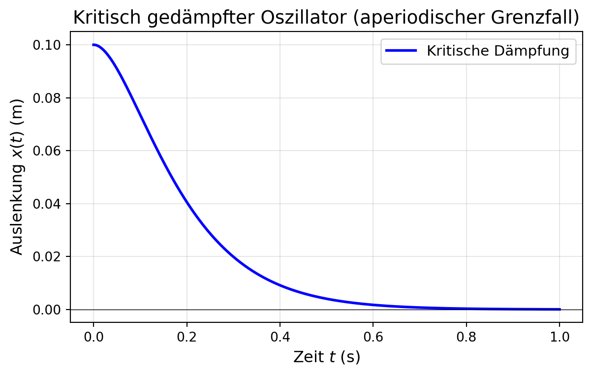
Das System mit kritischer Dämpfung \(c = 2\sqrt{mk} = 2\sqrt{1 \cdot 100} = 20\,\text{Ns/m}\).

Lösung

Für kritische Dämpfung gilt: \[ \gamma = \frac{20}{2} = 10\,\text{s}^{-1} = \omega_0 \]

Die charakteristische Gleichung hat eine Doppelwurzel \(\lambda = -\gamma = -10\). Die allgemeine Lösung lautet: \[ x(t) = (C_1 + C_2 t) e^{-\gamma t} \]

Mit den Anfangsbedingungen \(x(0) = 0.1\) und \(\dot{x}(0) = 0\) ergibt sich: \[ C_1 = 0.1, \quad C_2 = \gamma C_1 = 1 \]

Die Lösung ist: \[ x(t) = (0.1 + t) e^{-10t}\,\text{m} \]

import numpy as np
import matplotlib.pyplot as plt

# Parameter für kritische Dämpfung
m = 1.0
k = 100.0
c_crit = 2*np.sqrt(m*k)

omega_0 = np.sqrt(k/m)
gamma = c_crit/(2*m)

# Anfangsbedingungen
x0 = 0.1
v0 = 0.0

C1 = x0
C2 = v0 + gamma*x0

# Zeit
t = np.linspace(0, 1, 1000)

# Lösung
x_crit = (C1 + C2*t) * np.exp(-gamma*t)

plt.figure(figsize=(7, 4))
plt.plot(t, x_crit, 'b-', linewidth=2, label='Kritische Dämpfung')
plt.axhline(y=0, color='k', linestyle='-', linewidth=0.5)
plt.xlabel('Zeit $t$ (s)', fontsize=12)
plt.ylabel('Auslenkung $x(t)$ (m)', fontsize=12)
plt.title('Kritisch gedämpfter Oszillator (aperiodischer Grenzfall)', fontsize=14)
plt.grid(True, alpha=0.3)
plt.legend(fontsize=11)
plt.show()

Abbildung 3: Kritisch gedämpfter harmonischer Oszillator

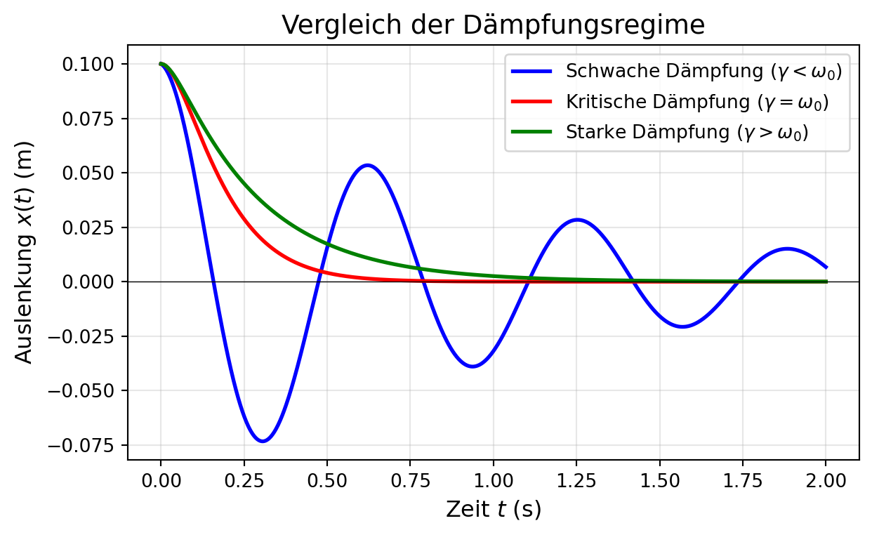
Beispiel 4: Vergleich der Dämpfungsregime

Wir vergleichen alle drei Regime mit denselben Anfangsbedingungen.

import numpy as np
import matplotlib.pyplot as plt

m = 1.0
k = 100.0
omega_0 = np.sqrt(k/m)

# Anfangsbedingungen
x0 = 0.1
v0 = 0.0

t = np.linspace(0, 2, 1000)

# Schwache Dämpfung
c_under = 2.0
gamma_under = c_under/(2*m)
omega_d = np.sqrt(omega_0**2 - gamma_under**2)
x_under = x0 * np.exp(-gamma_under*t) * np.cos(omega_d*t)

# Kritische Dämpfung
c_crit = 2*np.sqrt(m*k)
gamma_crit = c_crit/(2*m)
C1_crit = x0
C2_crit = v0 + gamma_crit*x0
x_crit = (C1_crit + C2_crit*t) * np.exp(-gamma_crit*t)

# Starke Dämpfung
c_over = 30.0
gamma_over = c_over/(2*m)
lambda1 = -gamma_over + np.sqrt(gamma_over**2 - omega_0**2)
lambda2 = -gamma_over - np.sqrt(gamma_over**2 - omega_0**2)
C2_over = (v0 - lambda1*x0)/(lambda2 - lambda1)
C1_over = x0 - C2_over
x_over = C1_over * np.exp(lambda1*t) + C2_over * np.exp(lambda2*t)

plt.figure(figsize=(7, 4))
plt.plot(t, x_under, 'b-', linewidth=2, label='Schwache Dämpfung ($\\gamma < \\omega_0$)')
plt.plot(t, x_crit, 'r-', linewidth=2, label='Kritische Dämpfung ($\\gamma = \\omega_0$)')
plt.plot(t, x_over, 'g-', linewidth=2, label='Starke Dämpfung ($\\gamma > \\omega_0$)')
plt.axhline(y=0, color='k', linestyle='-', linewidth=0.5)
plt.xlabel('Zeit $t$ (s)', fontsize=12)
plt.ylabel('Auslenkung $x(t)$ (m)', fontsize=12)
plt.title('Vergleich der Dämpfungsregime', fontsize=14)
plt.grid(True, alpha=0.3)
plt.legend(fontsize=10)
plt.show()

Abbildung 4: Vergleich der drei Dämpfungsregime

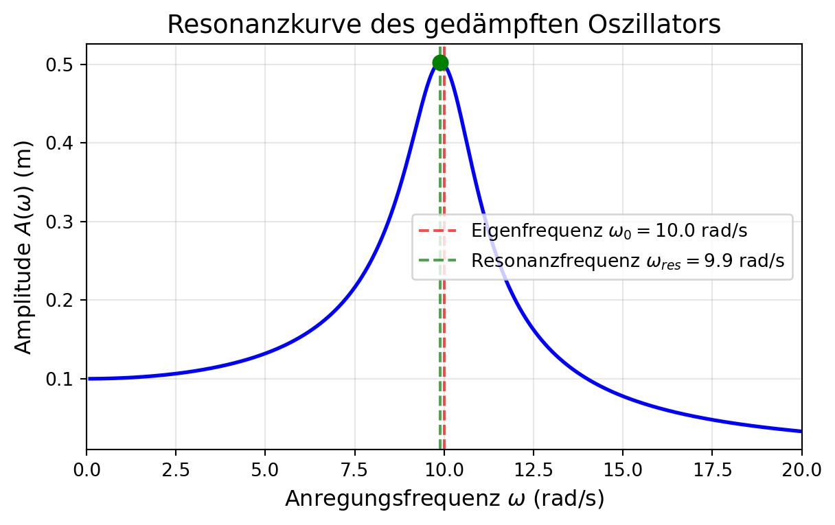
Beispiel 5: Resonanzkurve

Wir betrachten einen schwach gedämpften Oszillator unter harmonischer Anregung und untersuchen die Amplitude als Funktion der Anregungsfrequenz.

Parameter

\[ m = 1\,\text{kg}, \quad k = 100\,\text{N/m}, \quad c = 2\,\text{Ns/m}, \quad F_0 = 10\,\text{N} \]

Die Amplitude der stationären Schwingung ist: \[ A(\omega) = \frac{F_0/m}{\sqrt{(\omega_0^2 - \omega^2)^2 + (2\gamma\omega)^2}} \]

import numpy as np
import matplotlib.pyplot as plt

m = 1.0
k = 100.0
c = 2.0
F0 = 10.0

omega_0 = np.sqrt(k/m)
gamma = c/(2*m)

# Frequenzbereich
omega = np.linspace(0.1, 20, 1000)

# Amplitude
A = (F0/m) / np.sqrt((omega_0**2 - omega**2)**2 + (2*gamma*omega)**2)

# Resonanzfrequenz
omega_res = np.sqrt(omega_0**2 - 2*gamma**2)
A_res = (F0/m) / np.sqrt((omega_0**2 - omega_res**2)**2 + (2*gamma*omega_res)**2)

plt.figure(figsize=(7, 4))
plt.plot(omega, A, 'b-', linewidth=2)
plt.axvline(x=omega_0, color='r', linestyle='--', linewidth=1.5, alpha=0.7, label=f'Eigenfrequenz $\\omega_0 = {omega_0:.1f}$ rad/s')
plt.axvline(x=omega_res, color='g', linestyle='--', linewidth=1.5, alpha=0.7, label=f'Resonanzfrequenz $\\omega_{{res}} = {omega_res:.1f}$ rad/s')
plt.plot(omega_res, A_res, 'go', markersize=8)
plt.xlabel('Anregungsfrequenz $\\omega$ (rad/s)', fontsize=12)
plt.ylabel('Amplitude $A(\\omega)$ (m)', fontsize=12)
plt.title('Resonanzkurve des gedämpften Oszillators', fontsize=14)
plt.grid(True, alpha=0.3)
plt.legend(fontsize=10)
plt.xlim([0, 20])
plt.show()

Abbildung 5: Resonanzkurve: Amplitude als Funktion der Anregungsfrequenz

Die Resonanzkurve zeigt das Maximum der Amplitude bei der Resonanzfrequenz. Bei schwacher Dämpfung liegt diese nahe der Eigenfrequenz. Je stärker die Dämpfung, desto breiter und flacher wird das Resonanzmaximum.