Nichtlineare DGLs

NoteLernziele

Die Studierenden sollen…

• … die Unterschiede zwischen linearen und nichtlinearen Differentialgleichungen erklären und Beispiele für nichtlineares Verhalten nennen können.

• … das logistische Wachstumsmodell herleiten und durch Separation der Variablen lösen können.

• … Gleichgewichtspunkte nichtlinearer Systeme finden und deren Stabilität durch Linearisierung analysieren können.

• … das Lotka-Volterra-Modell auf Räuber-Beute-Systeme anwenden und periodische Oszillationen interpretieren können.

Einführung in nichtlineare Differentialgleichungen

In den bisherigen Kapiteln haben wir uns hauptsächlich mit linearen Differentialgleichungen beschäftigt. Diese besitzen die angenehme Eigenschaft, dass das Superpositionsprinzip gilt. Die Summe zweier Lösungen ist wieder eine Lösung, und Lösungen lassen sich mit Konstanten multiplizieren. Diese mathematische Eleganz hat jedoch ihren Preis: Lineare Differentialgleichungen sind idealisierte Modelle, die reale Phänomene oft nur näherungsweise beschreiben.

Die meisten natürlichen Prozesse sind fundamental nichtlinear. Eine Differentialgleichung heißt nichtlinear, wenn sie Terme enthält, die nicht linear in der gesuchten Funktion und ihren Ableitungen sind. Beispiele für solche Terme sind Produkte wie \(y^2\), \(y\dot{y}\) oder \(xy\), aber auch nichtlineare Funktionen wie \(\sin(y)\) oder \(e^y\). Diese Nichtlinearitäten mögen auf den ersten Blick wie kleine Komplikationen erscheinen, aber sie führen zu qualitativ neuem und oft überraschendem Verhalten.

Nichtlineare Differentialgleichungen können Phänomene zeigen, die bei linearen Gleichungen unmöglich sind. Dazu gehören multiple stabile Zustände, bei denen das System je nach Anfangsbedingung in unterschiedlichen Gleichgewichten endet. Periodische Oszillationen können spontan entstehen, ohne dass eine externe periodische Kraft wirkt. In manchen Fällen zeigt das System sogar chaotisches Verhalten, bei dem winzige Änderungen der Anfangsbedingungen zu völlig anderen Verläufen führen.

Die mathematische Behandlung nichtlinearer Gleichungen ist erheblich schwieriger als bei linearen. Es gibt keine allgemeinen Lösungsformeln, und selbst für einfach aussehende nichtlineare Gleichungen existiert oft keine analytische Lösung in geschlossener Form. Stattdessen sind wir auf numerische Methoden und qualitative Analysetechniken angewiesen. Trotz dieser Schwierigkeiten ist das Studium nichtlinearer Differentialgleichungen unverzichtbar, denn nur sie können die Komplexität realer Systeme adäquat beschreiben.

Logistisches Wachstum

Ein klassisches Beispiel für eine nichtlineare Differentialgleichung ist das logistische Wachstumsmodell. Es beschreibt das Wachstum einer Population unter Berücksichtigung begrenzter Ressourcen und überwindet damit die Unrealistik des exponentiellen Wachstumsmodells.

Herleitung des Modells

Das einfachste Populationsmodell ist das Malthus-Modell, das exponentielles Wachstum postuliert. Es besagt, dass die Änderungsrate der Populationsgröße proportional zur aktuellen Population ist: \[ \frac{\mathrm{d}y}{\mathrm{d}t} = ry \tag{1}\]

Hierbei ist \(r\) die intrinsische Wachstumsrate, die die Differenz zwischen Geburten- und Sterberate repräsentiert. Die Lösung dieser Gleichung ist \(y(t) = y_0 e^{rt}\), was unbegrenztes exponentielles Wachstum beschreibt.

In der Realität kann keine Population unbegrenzt wachsen. Limitierende Faktoren wie Nahrungsmangel, Platzmangel, Ansammlung von Abfallprodukten oder Krankheiten bremsen das Wachstum. Diese Effekte werden umso stärker, je näher die Population einer kritischen Größe kommt, die man als Umweltkapazität oder Tragfähigkeit bezeichnet.

Um diese Sättigung zu modellieren, führen wir einen Hemmfaktor ein, der mit zunehmender Populationsgröße stärker wird. Der einfachste Ansatz ist ein linearer Hemmfaktor der Form \(1 - y/K\), wobei \(K\) die Umweltkapazität darstellt. Für kleine Populationen (\(y \ll K\)) ist dieser Faktor nahe bei eins und das Wachstum approximiert das Malthus-Modell. Für Populationen nahe der Kapazität (\(y \approx K\)) verschwindet der Faktor und das Wachstum stoppt.

Durch Multiplikation der Malthus-Gleichung mit diesem Hemmfaktor erhalten wir die logistische Gleichung: \[ \frac{\mathrm{d}y}{\mathrm{d}t} = ry\left(1 - \frac{y}{K}\right) \tag{2}\]

Diese Gleichung ist nichtlinear wegen des Produkts \(y \cdot y/K = y^2/K\). Trotz dieser Nichtlinearität lässt sie sich analytisch lösen.

Gleichgewichtspunkte und Stabilität

Gleichgewichtspunkte oder Fixpunkte sind Zustände, in denen die Population konstant bleibt, also \(\mathrm{d}y/\mathrm{d}t = 0\) gilt. Für die logistische Gleichung bedeutet dies: \[ ry\left(1 - \frac{y}{K}\right) = 0 \]

Dies führt auf zwei Gleichgewichte: \(y^* = 0\) und \(y^* = K\). Das erste entspricht dem Aussterben der Population, das zweite der Sättigung bei Umweltkapazität.

Um die Stabilität dieser Gleichgewichte zu untersuchen, betrachten wir kleine Störungen. Sei \(y(t) = y^* + \varepsilon(t)\) mit kleinem \(\varepsilon\). Einsetzen in die Differentialgleichung und Linearisierung ergibt: \[ \frac{\mathrm{d}\varepsilon}{\mathrm{d}t} \approx f'(y^*) \varepsilon \]

wobei \(f(y) = ry(1 - y/K)\) und \(f'(y) = r(1 - 2y/K)\). Die Stabilität wird durch das Vorzeichen von \(f'(y^*)\) bestimmt.

Am Gleichgewicht \(y^* = 0\) gilt \(f'(0) = r > 0\). Die Störung wächst exponentiell, das Gleichgewicht ist instabil. Eine kleine Population wird nicht gegen null gehen, sondern wachsen. Am Gleichgewicht \(y^* = K\) gilt \(f'(K) = -r < 0\). Störungen klingen exponentiell ab, das Gleichgewicht ist stabil. Eine Population nahe der Kapazität wird zu dieser zurückkehren.

Dieses Stabilitätsverhalten lässt sich anschaulich im Richtungsfeld der logistischen Gleichung erkennen, das in Abbildung 1 gezeigt ist. Alle Lösungskurven werden vom instabilen Gleichgewicht \(y = 0\) weggetrieben und vom stabilen Gleichgewicht \(y = K\) angezogen.

import numpy as np
import matplotlib.pyplot as plt

# Parameter
r = 1.0  # Wachstumsrate
K = 1.0  # Umweltkapazität

fig, ax = plt.subplots(figsize=(7, 4))

# Gitter für das Richtungsfeld
T, Y = np.meshgrid(np.linspace(0, 8, 25), np.linspace(-0.1, 1.6, 22))
dY = r * Y * (1 - Y / K)
dT = np.ones_like(dY)

# Normierung der Pfeile auf einheitliche Länge
norm = np.sqrt(dT**2 + dY**2)
ax.quiver(T, Y, dT / norm, dY / norm, angles='xy', color='gray', alpha=0.6,
          scale=35, width=0.002, headwidth=4)

# Lösungskurven für verschiedene Anfangswerte
t = np.linspace(0, 8, 400)
for y0 in [0.05, 0.2, 0.5, 1.2, 1.5]:
    y = K / (1 + (K / y0 - 1) * np.exp(-r * t))
    ax.plot(t, y, linewidth=2, label=f'$y_0 = {y0}$')

# Gleichgewichte
ax.axhline(y=0, color='red', linestyle='--', linewidth=1.5, label='$y = 0$ (instabil)')
ax.axhline(y=K, color='green', linestyle='--', linewidth=1.5, label=f'$y = K = {K:.0f}$ (stabil)')

ax.set_xlabel('Zeit $t$', fontsize=12)
ax.set_ylabel('Population $y$', fontsize=12)
ax.set_title('Richtungsfeld der logistischen Gleichung', fontsize=12)
ax.grid(True, alpha=0.3)
ax.legend(fontsize=9, loc='center right')
ax.set_xlim([0, 8])
ax.set_ylim([-0.1, 1.6])

plt.tight_layout()
plt.show()

Abbildung 1: Richtungsfeld der logistischen Gleichung für \(r = 1\) und \(K = 1\) mit Lösungskurven für Anfangswerte unter und über der Kapazität \(K\). Die gestrichelten Linien markieren die Gleichgewichte \(y = 0\) (instabil) und \(y = K\) (stabil).

Analytische Lösung

Obwohl die logistische Gleichung nichtlinear ist, lässt sie sich durch Separation der Variablen lösen. Wir schreiben: \[ \frac{\mathrm{d}y}{y(1 - y/K)} = r \, \mathrm{d}t \]

Die linke Seite kann durch Partialbruchzerlegung umgeformt werden: \[ \frac{1}{y(1 - y/K)} = \frac{1}{y} + \frac{1/K}{1 - y/K} \]

Integration beider Seiten führt nach einigen Umformungen auf die Lösung: \[ y(t) = \frac{K}{1 + \left(\frac{K}{y_0} - 1\right)e^{-rt}} \tag{3}\]

wobei \(y_0 = y(0)\) die Anfangspopulation ist. Für \(t \to \infty\) strebt \(y(t) \to K\), unabhängig vom Anfangswert \(y_0 > 0\). Die Population nähert sich asymptotisch der Kapazität.

Diese Lösung zeigt charakteristisches sigmoidales Verhalten. Für kleine Zeiten und \(y_0 \ll K\) wächst die Population annähernd exponentiell. Für mittlere Zeiten ist das Wachstum maximal. Für große Zeiten verlangsamt sich das Wachstum und die Population sättigt bei \(K\).

Visualisierung

Die folgende Grafik zeigt die Populationsentwicklung für verschiedene Anfangsbedingungen sowie das Phasenporträt der logistischen Gleichung.

import numpy as np
import matplotlib.pyplot as plt

# Parameter
r = 0.5  # Wachstumsrate
K = 100  # Umweltkapazität

# Zeit
t = np.linspace(0, 20, 1000)

# Verschiedene Anfangsbedingungen
y0_values = [5, 50, 120, 150]

fig, axes = plt.subplots(1, 2, figsize=(7, 4))

# === Linke Seite: Zeitverlauf ===
ax = axes[0]
for y0 in y0_values:
    y = K / (1 + (K / y0 - 1) * np.exp(-r * t))
    ax.plot(t, y, linewidth=2, label=f'$y_0 = {y0}$')

ax.axhline(y=K, color='red', linestyle='--', linewidth=2, label=f'Kapazität $K = {K}$')
ax.axhline(y=0, color='gray', linestyle=':', alpha=0.5)
ax.set_xlabel('Zeit $t$', fontsize=12)
ax.set_ylabel('Population $y(t)$', fontsize=12)
ax.set_title('Logistisches Wachstum: Zeitverlauf', fontsize=12)
ax.grid(True, alpha=0.3)
ax.legend(fontsize=10)

# === Rechte Seite: Phasenporträt ===
ax = axes[1]
y = np.linspace(0, 150, 1000)
dy_dt = r * y * (1 - y / K)

ax.plot(y, dy_dt, 'b-', linewidth=2.5, label='$\\frac{\mathrm{d}y}{\mathrm{d}t} = ry(1 - y/K)$')
ax.axhline(y=0, color='k', linewidth=0.5)
ax.plot([0, K], [0, 0], 'ro', markersize=10, label='Gleichgewichtspunkte')
ax.fill_between(y, 0, dy_dt, where=(dy_dt > 0), alpha=0.2, color='green', label='Wachstum')
ax.fill_between(y, 0, dy_dt, where=(dy_dt < 0), alpha=0.2, color='red', label='Rückgang')

ax.set_xlabel('Population $y$', fontsize=12)
ax.set_ylabel('$\\frac{\mathrm{d}y}{\mathrm{d}t}$', fontsize=12)
ax.set_title('Phasenporträt (1D)', fontsize=12)
ax.grid(True, alpha=0.3)
ax.legend(fontsize=10)
ax.set_xlim([0, 150])

plt.tight_layout()
plt.show()

Abbildung 2: Logistisches Wachstumsmodell: Populationsentwicklung für verschiedene Anfangsbedingungen

Die linke Grafik zeigt, dass alle Populationen mit \(y_0 > 0\) gegen die Kapazität \(K\) konvergieren. Populationen, die initial über der Kapazität liegen, schrumpfen auf \(K\). Das rechte Phasenporträt visualisiert die Wachstumsrate als Funktion der Population. Die Wachstumsrate ist maximal bei \(y = K/2\) und verschwindet an den beiden Gleichgewichtspunkten.

Räuber-Beute-Systeme

Während die logistische Gleichung eine einzelne Population beschreibt, betrachten wir nun die Wechselwirkung zweier Populationen. Das Lotka-Volterra-Modell ist das klassische Beispiel für ein System gekoppelter nichtlinearer Differentialgleichungen und beschreibt die Dynamik zwischen Räuber und Beute.

Herleitung des Räuber-Beute-Modells

Betrachten wir zunächst die Beute-Population, etwa Hasen, in Abwesenheit von Räubern. Bei unbegrenzten Ressourcen würde sie exponentiell wachsen: \[ \frac{\mathrm{d}x}{\mathrm{d}t} = \alpha x \tag{4}\]

Hierbei ist \(\alpha > 0\) die intrinsische Wachstumsrate der Beute. Ohne Nahrung würde die Räuber-Population, etwa Luchse, exponentiell schrumpfen: \[ \frac{\mathrm{d}y}{\mathrm{d}t} = -\gamma y \tag{5}\]

wobei \(\gamma > 0\) die natürliche Sterberate der Räuber ist.

Die Wechselwirkung zwischen Räuber und Beute geschieht durch Jagd. Die Rate der Begegnungen zwischen beiden Spezies ist proportional zum Produkt ihrer Populationsgrößen, \(xy\). Dies ist eine nichtlineare Kopplung. Jede solche Begegnung bedeutet im Mittel den Tod einer Beute und die Nahrungsaufnahme eines Räubers.

Der Verlust der Beute durch Jagd ist proportional zu \(\beta xy\), wobei \(\beta\) die Prädationsrate ist. Der Gewinn der Räuber durch Nahrungsaufnahme ist proportional zu \(\delta xy\), wobei \(\delta\) die Konversionseffizienz beschreibt, mit der verzehrte Beute in Räubernachkommen umgesetzt wird.

Kombiniert man diese Effekte, erhält man das Lotka-Volterra-Modell: \[ \begin{aligned} \frac{\mathrm{d}x}{\mathrm{d}t} &= \alpha x - \beta xy \\ \frac{\mathrm{d}y}{\mathrm{d}t} &= \delta xy - \gamma y \end{aligned} \tag{6}\]

Dieses System ist nichtlinear wegen der Produktterme \(xy\) in beiden Gleichungen. Die Parameter \(\alpha\), \(\beta\), \(\gamma\) und \(\delta\) sind alle positiv.

Gleichgewichtspunkte

Gleichgewichtspunkte erfüllen \(\mathrm{d}x/\mathrm{d}t = 0\) und \(\mathrm{d}y/\mathrm{d}t = 0\). Aus den Gleichungen folgt: \[ \begin{aligned} x(\alpha - \beta y) &= 0 \\ y(\delta x - \gamma) &= 0 \end{aligned} \]

Dies ergibt zwei Gleichgewichte. Das triviale Gleichgewicht \((x^*, y^*) = (0, 0)\) entspricht dem Aussterben beider Populationen. Das nichttriviale Gleichgewicht liegt bei: \[ (x^*, y^*) = \left(\frac{\gamma}{\delta}, \frac{\alpha}{\beta}\right) \tag{7}\]

Bemerkenswerterweise hängt die Gleichgewichtsgröße der Beute-Population nur von den Räuber-Parametern \(\gamma\) und \(\delta\) ab. Ebenso hängt die Gleichgewichtsgröße der Räuber nur von den Beute-Parametern \(\alpha\) und \(\beta\) ab.

Periodische Oszillationen

Das Lotka-Volterra-System besitzt eine Erhaltungsgröße oder ein erstes Integral: \[ H(x, y) = \delta x - \gamma \ln x + \beta y - \alpha \ln y = \text{const} \tag{8}\]

Die Existenz dieser Erhaltungsgröße bedeutet, dass sich das System entlang von Niveaulinien von \(H\) bewegt. Diese Niveaulinien sind geschlossene Kurven um das Gleichgewicht. Das System zeigt daher periodische Oszillationen.

Die physikalische Interpretation dieser Oszillationen ist aufschlussreich. Startet man mit vielen Beutetieren und wenigen Räubern, so finden die Räuber reichlich Nahrung und vermehren sich. Die wachsende Räuberpopulation dezimiert die Beute. Wenn die Beute knapp wird, verhungern die Räuber. Mit wenigen Räubern kann sich die Beute wieder erholen, und der Zyklus beginnt von neuem.

Linearisierung und Stabilität

Um die Stabilität des Gleichgewichts zu untersuchen, berechnen wir die Jacobi-Matrix: \[ J(x, y) = \begin{pmatrix} \alpha - \beta y & -\beta x \\ \delta y & \delta x - \gamma \end{pmatrix} \]

Am Gleichgewicht \((x^*, y^*) = (\gamma/\delta, \alpha/\beta)\) ergibt sich: \[ J^* = \begin{pmatrix} 0 & -\beta \gamma/\delta \\ \delta \alpha/\beta & 0 \end{pmatrix} \]

Die Spur dieser Matrix ist \(\tau = 0\) und die Determinante ist \(\Delta = \alpha \gamma > 0\). Die Eigenwerte sind daher \(\lambda = \pm i\sqrt{\alpha \gamma}\), also rein imaginär. Dies entspricht dem Grenzfall zwischen Stabilität und Instabilität und erklärt die periodischen Oszillationen.

Das Gleichgewicht ist neutral stabil. Kleine Störungen führen weder zu Konvergenz zum Gleichgewicht noch zu Divergenz, sondern zu periodischen Bewegungen um das Gleichgewicht herum. Die Amplitude dieser Oszillationen hängt von der Größe der Störung ab.

Visualisierung der Räuber-Beute-Dynamik

Die folgende Grafik zeigt die charakteristischen geschlossenen Orbits in der Phasenebene sowie die periodischen Populationsschwankungen über die Zeit.

import numpy as np
import matplotlib.pyplot as plt
from scipy.integrate import solve_ivp

# Parameter
alpha = 1.0  # Wachstumsrate Beute
beta = 0.5   # Prädationsrate
gamma = 1.0  # Sterberate Räuber
delta = 0.5  # Effizienz der Prädation

# Gleichgewicht
x_eq = gamma / delta
y_eq = alpha / beta

# System der Differentialgleichungen
def lotka_volterra(t, y):
    x, y_pred = y
    dx = alpha * x - beta * x * y_pred
    dy = delta * x * y_pred - gamma * y_pred
    return [dx, dy]

# Verschiedene Anfangsbedingungen
initial_conditions = [
    (0.5, 0.5),
    (1.0, 1.0),
    (2.0, 0.8),
    (0.8, 2.0),
]

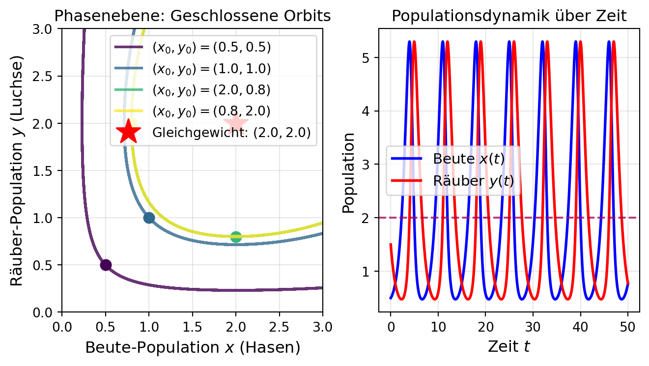
fig, axes = plt.subplots(1, 2, figsize=(7, 4))

# === Linke Seite: Phasenebene ===
ax = axes[0]
colors = plt.cm.viridis(np.linspace(0, 1, len(initial_conditions)))

for (x0, y0), color in zip(initial_conditions, colors):
    sol = solve_ivp(lotka_volterra, [0, 100], [x0, y0], dense_output=True, max_step=0.1)
    ax.plot(sol.y[0], sol.y[1], color=color, linewidth=2, alpha=0.8, label=f'$(x_0, y_0) = ({x0}, {y0})$')
    ax.plot(x0, y0, 'o', color=color, markersize=8)

# Nullklinen: dx/dt = 0 auf y = alpha/beta, dy/dt = 0 auf x = gamma/delta
ax.axhline(y=y_eq, color='gray', linestyle='--', linewidth=1.5,
           label=f'Nullkline $y = \\alpha/\\beta = {y_eq:.1f}$')
ax.axvline(x=x_eq, color='gray', linestyle='-.', linewidth=1.5,
           label=f'Nullkline $x = \\gamma/\\delta = {x_eq:.1f}$')

# Gleichgewichtspunkt
ax.plot(x_eq, y_eq, 'r*', markersize=20, label=f'Gleichgewicht: $({x_eq:.1f}, {y_eq:.1f})$')

ax.set_xlabel('Beute-Population $x$ (Hasen)', fontsize=12)
ax.set_ylabel('Räuber-Population $y$ (Luchse)', fontsize=12)
ax.set_title('Phasenebene: Geschlossene Orbits', fontsize=12)
ax.grid(True, alpha=0.3)
ax.legend(fontsize=8)
ax.set_xlim([0, 3])
ax.set_ylim([0, 3])

# === Rechte Seite: Zeitverlauf ===
ax = axes[1]
x0, y0 = 0.5, 1.5
sol = solve_ivp(lotka_volterra, [0, 50], [x0, y0], dense_output=True, max_step=0.01)

ax.plot(sol.t, sol.y[0], 'b-', linewidth=2, label='Beute $x(t)$')
ax.plot(sol.t, sol.y[1], 'r-', linewidth=2, label='Räuber $y(t)$')
ax.axhline(y=x_eq, color='b', linestyle='--', alpha=0.5)
ax.axhline(y=y_eq, color='r', linestyle='--', alpha=0.5)

ax.set_xlabel('Zeit $t$', fontsize=12)
ax.set_ylabel('Population', fontsize=12)
ax.set_title('Populationsdynamik über Zeit', fontsize=12)
ax.grid(True, alpha=0.3)
ax.legend(fontsize=11)

plt.tight_layout()
plt.show()

Abbildung 3: Lotka-Volterra-Modell: Räuber-Beute-Dynamik. Im Phasenporträt (links) sind zusätzlich die Nullklinen \(y = \alpha/\beta\) und \(x = \gamma/\delta\) (gestrichelt) eingezeichnet, deren Schnittpunkt das nichttriviale Gleichgewicht ist.

Die linke Grafik zeigt die geschlossenen Orbits in der Phasenebene. Jede Anfangsbedingung führt zu einer periodischen Trajektorie, deren Form und Amplitude von der Energie der Erhaltungsgröße abhängt. Die rechte Grafik zeigt den zeitlichen Verlauf der Populationen. Die Oszillationen von Räuber und Beute sind phasenverschoben: Das Maximum der Beutepopulation geht dem Maximum der Räuberpopulation voraus.

Stabilitätsanalyse nichtlinearer Systeme

Die allgemeine Analyse nichtlinearer Systeme erfordert Techniken, die über die direkte Lösung hinausgehen. Die Linearisierung um Gleichgewichtspunkte ist eine mächtige Methode, die lokale Aussagen über das Systemverhalten ermöglicht.

Linearisierung um Gleichgewichtspunkte

Betrachten wir ein allgemeines nichtlineares System: \[ \dot{\mathbf{y}} = \mathbf{f}(\mathbf{y}) \tag{9}\]

Ein Gleichgewichtspunkt \(\mathbf{y}^*\) erfüllt \(\mathbf{f}(\mathbf{y}^*) = \mathbf{0}\). Um das Verhalten in der Nähe dieses Gleichgewichts zu verstehen, schreiben wir \(\mathbf{y}(t) = \mathbf{y}^* + \mathbf{u}(t)\) mit einer kleinen Störung \(\mathbf{u}(t)\).

Einsetzen in die Differentialgleichung und Taylor-Entwicklung nach \(\mathbf{u}\) ergibt: \[ \dot{\mathbf{u}} = \mathbf{f}(\mathbf{y}^* + \mathbf{u}) \approx \mathbf{f}(\mathbf{y}^*) + J(\mathbf{y}^*) \mathbf{u} + O(\|\mathbf{u}\|^2) \]

Da \(\mathbf{f}(\mathbf{y}^*) = \mathbf{0}\) und wir nur die lineare Näherung betrachten, erhalten wir: \[ \dot{\mathbf{u}} \approx J(\mathbf{y}^*) \mathbf{u} \tag{10}\]

Hierbei ist \(J(\mathbf{y}^*)\) die Jacobi-Matrix, die Matrix aller partiellen Ableitungen: \[ J(\mathbf{y}) = \begin{pmatrix} \frac{\partial f_1}{\partial y_1} & \cdots & \frac{\partial f_1}{\partial y_n} \\ \vdots & \ddots & \vdots \\ \frac{\partial f_n}{\partial y_1} & \cdots & \frac{\partial f_n}{\partial y_n} \end{pmatrix} \tag{11}\]

Das linearisierte System ist ein lineares System mit konstanten Koeffizienten, dessen Verhalten durch die Eigenwerte von \(J(\mathbf{y}^*)\) bestimmt wird.

Stabilitätskriterien für zweidimensionale Systeme

Für ein zweidimensionales System mit Jacobi-Matrix \[ J = \begin{pmatrix} a & b \\ c & d \end{pmatrix} \] sind zwei Größen besonders wichtig: die Spur \(\tau = a + d\) und die Determinante \(\Delta = ad - bc\). Die Eigenwerte sind: \[ \lambda = \frac{\tau \pm \sqrt{\tau^2 - 4\Delta}}{2} \]

Die Stabilität des Gleichgewichts wird durch Spur und Determinante vollständig charakterisiert. Ist \(\Delta < 0\), so haben die Eigenwerte unterschiedliche Vorzeichen. Das Gleichgewicht ist ein Sattelpunkt und instabil. Ist \(\Delta > 0\) und \(\tau < 0\), so sind beide Realteile negativ. Das Gleichgewicht ist stabil und Trajektorien konvergieren zu ihm.

Für \(\Delta > 0\) und \(\tau = 0\) liegen die Eigenwerte auf der imaginären Achse. Das Gleichgewicht ist neutral stabil und das System zeigt periodische Bewegungen. Dies ist der Fall beim Lotka-Volterra-System. Für \(\Delta > 0\) und \(\tau > 0\) ist das Gleichgewicht instabil und Trajektorien divergieren.

Die Form der Diskriminante \(\tau^2 - 4\Delta\) bestimmt, ob die Eigenwerte reell oder komplex sind. Reelle Eigenwerte entsprechen exponentiellen Moden ohne Oszillation. Komplexe Eigenwerte führen zu spiralförmigen Trajektorien mit gleichzeitiger Oszillation und exponentiellem Wachstum oder Zerfall.

Zusammenfassung

Nichtlineare Differentialgleichungen zeigen qualitativ neuartiges Verhalten im Vergleich zu linearen Systemen. Das Superpositionsprinzip gilt nicht mehr, und die Dynamik kann multiple stabile Zustände, spontane Oszillationen und sogar Chaos umfassen. Diese Komplexität macht nichtlineare Systeme sowohl schwieriger zu analysieren als auch interessanter für die Modellierung realer Phänomene.

Das logistische Wachstumsmodell ist ein einfaches Beispiel, das trotz Nichtlinearität analytisch lösbar ist. Es zeigt, wie ein Sättigungseffekt aus einer nichtlinearen Modifikation des exponentiellen Wachstums entsteht. Das Lotka-Volterra-Modell demonstriert die Komplexität gekoppelter nichtlinearer Systeme. Die Wechselwirkung zwischen Räuber und Beute führt zu periodischen Oszillationen, die durch eine Erhaltungsgröße charakterisiert sind.

Die Linearisierung um Gleichgewichtspunkte ist eine zentrale Methode zur Analyse nichtlinearer Systeme. Durch Berechnung der Jacobi-Matrix und ihrer Eigenwerte lässt sich die lokale Stabilität bestimmen. Diese lokale Analyse liefert wichtige Einsichten, auch wenn sie das globale Verhalten nicht vollständig erfassen kann. Für ein umfassendes Verständnis sind numerische Simulationen und geometrische Methoden wie die Phasenraumanalyse unverzichtbar.