Konzepte

Lernziele

Die Studierenden sollen…

… das Hamilton-Prinzip der kleinsten Wirkung erläutern und die Lagrangefunktion mechanischer Systeme angeben können.

… aus der Lagrangefunktion systematisch die Euler-Lagrange-Gleichungen für mechanische Systeme erstellen können.
… dissipative Systeme mit der Rayleigh-Dissipationsfunktion in den Lagrange-Formalismus einbeziehen können.

… die mechanisch-elektrische Analogie in Beziehung setzen und Entsprechungen zwischen mechanischen und elektrischen Größen angeben können.

Einführung: Von der Variationsrechnung zu Differentialgleichungen

Die Verbindung zwischen Variationsrechnung und Differentialgleichungen eröffnet eine völlig neue Perspektive auf die Dynamik physikalischer Systeme. Anstatt einzelne Kräfte zu identifizieren und gemäß den Newtonschen Gesetzen aufzuaddieren, können wir die Bewegung als Optimierungsproblem formulieren. Die Natur wählt in gewissem Sinne den Weg, der ein bestimmtes Funktional extremal macht.

Diese Perspektive, die ursprünglich von Leibniz, Maupertuis und Euler entwickelt und später von Lagrange und Hamilton perfektioniert wurde, führt zu einer universellen Methode zur Herleitung von Bewegungsgleichungen. Der große Vorteil dieser Methode liegt in ihrer Allgemeinheit und Eleganz. Sie funktioniert für beliebige Koordinatensysteme und lässt sich auf komplexe Systeme mit vielen Freiheitsgraden anwenden.

Das Hamilton-Prinzip, auch Prinzip der kleinsten Wirkung genannt, bildet die konzeptionelle Grundlage. Zusammen mit der Variationsrechnung liefert es eine systematische Prozedur zur Herleitung der Bewegungsgleichungen dynamischer Systeme. Diese Gleichungen sind Differentialgleichungen, die das zeitliche Verhalten des Systems vollständig beschreiben.

Die Lagrangefunktion und die Wirkung

Der Ausgangspunkt der Lagrangeschen Mechanik ist die Lagrangefunktion. Sie fasst die gesamte Dynamik eines mechanischen Systems in einer einzigen skalaren Funktion zusammen und bildet die Grundlage für die Herleitung der Bewegungsgleichungen.

Definition der Lagrangefunktion

Die Lagrangefunktion eines mechanischen Systems ist typischerweise definiert als: \[ L = T^* - V \tag{1}\]

Hierbei bezeichnet \(T^*\) die kinetische Koenergie und \(V\) die potentielle Energie des Systems. Die kinetische Koenergie ist für ein System mit Geschwindigkeiten \(\dot{q}_i\) gegeben durch: \[ T^* = \frac{1}{2}\sum_i m_i \dot{q}_i^2 \tag{2}\]

Die potentielle Energie \(V\) hängt von den Positionen \(q_i\) ab und beschreibt die in Feldern oder elastischen Elementen gespeicherte Energie.

Die Wahl der Koordinaten \(q_i\) ist flexibel. Sie können kartesische Koordinaten, Winkel, Längen oder andere geeignete Größen sein, die die Konfiguration des Systems eindeutig beschreiben. Diese Koordinaten werden als generalisierte Koordinaten bezeichnet.

Die Wirkung als Zeitintegral

Die Wirkung ist ein Funktional, das der gesamten Bewegung eines Systems eine Zahl zuordnet. Sie ist definiert als das Zeitintegral der Lagrangefunktion: \[ S = \int_{t_1}^{t_2} L(t, q, \dot{q}) \, \mathrm{d}t \tag{3}\]

Die Wirkung hängt von der Trajektorie des Systems im Konfigurationsraum ab. Verschiedene mögliche Bewegungen zwischen zwei Zeitpunkten \(t_1\) und \(t_2\) führen zu verschiedenen Werten der Wirkung. Die tatsächliche Bewegung ist diejenige, die die Wirkung stationär macht.

Die Einheit der Wirkung ist Energie mal Zeit, also Joule-Sekunden. In der Quantenmechanik spielt die Wirkung eine zentrale Rolle, da das Plancksche Wirkungsquantum \(\hbar\) die fundamentale Skala für die Wirkung definiert.

Das Hamilton-Prinzip

Das Hamilton-Prinzip ist die fundamentale Aussage, die die Variationsrechnung mit der Mechanik verbindet. Es postuliert, dass die tatsächliche Bewegung eines physikalischen Systems durch die Stationarität der Wirkung charakterisiert ist.

Formulierung des Prinzips

Das Hamilton-Prinzip besagt, dass die Wirkung \(S\) für die tatsächliche Bewegung stationär ist: \[ \delta S = 0 \tag{4}\]

Diese Bedingung bedeutet, dass infinitesimale Variationen der Trajektorie die Wirkung nicht ändern. Die tatsächliche Bewegung ist ein Extremum des Wirkungsfunktionals unter allen möglichen Bewegungen mit denselben Anfangs- und Endbedingungen.

Das Prinzip ist bemerkenswert allgemein. Es gilt nicht nur für mechanische Systeme, sondern auch für Felder, Flüssigkeiten und sogar für die Elektrodynamik. Jede fundamentale physikalische Theorie lässt sich durch ein entsprechendes Wirkungsfunktional formulieren.

Die Stationarität der Wirkung ist eine notwendige Bedingung für ein Extremum. In den meisten physikalischen Anwendungen handelt es sich tatsächlich um ein Minimum, weshalb das Prinzip häufig als Prinzip der kleinsten Wirkung bezeichnet wird. Es gibt jedoch auch Fälle, in denen die Wirkung einen Sattelpunkt erreicht. Abbildung 1 veranschaulicht das Prinzip: Unter allen denkbaren Bahnen zwischen denselben festen Endpunkten zeichnet die Stationarität der Wirkung die tatsächlich durchlaufene Bahn aus.

Abbildung 1: Das Hamilton-Prinzip: Unter allen Bahnen \(q(t)\), die dieselben festen Endpunkte \(q(t_1)\) und \(q(t_2)\) verbinden (gestrichelt: variierte Bahnen \(q + \delta q\)), macht die tatsächlich durchlaufene Bahn die Wirkung stationär, \(\delta S = 0\).

Die allgemeinen Euler-Lagrange-Gleichungen

Aus dem Hamilton-Prinzip \(\delta S = 0\) folgen durch Anwendung der Variationsrechnung die Euler-Lagrange-Gleichungen. Für ein System mit \(n\) generalisierten Koordinaten \(q_i\) ergeben sich \(n\) gekoppelte Differentialgleichungen: \[ \frac{\partial L}{\partial q_i} - \frac{\mathrm{d}}{\mathrm{d}t}\left(\frac{\partial L}{\partial \dot{q}_i}\right) = 0, \quad i = 1, \ldots, n \tag{5}\]

Diese Gleichungen sind gewöhnliche Differentialgleichungen zweiter Ordnung für die Koordinaten \(q_i(t)\). Sie bilden ein System gekoppelter Differentialgleichungen, das die gesamte Dynamik des physikalischen Systems beschreibt.

Die Struktur dieser Gleichungen ist universell. Sie gilt unabhängig davon, ob wir ein mechanisches System, ein elektrisches Netzwerk oder ein anderes physikalisches System betrachten. Die spezifische Form der Bewegungsgleichungen ergibt sich erst, wenn wir die konkrete Lagrangefunktion einsetzen.

Generalisierte Koordinaten

Generalisierte Koordinaten sind beliebige Parameter, die den Zustand eines Systems vollständig beschreiben. Sie müssen keine kartesischen Koordinaten sein — sie können jede physikalische Größe repräsentieren, die sich zeitlich ändern kann:

System	Generalisierte Koordinate	Bedeutung
Masse an Feder	Position \(x\)	Auslenkung aus der Ruhelage
Pendel	Winkel \(\theta\)	Auslenkung aus der Vertikalen
LC-Schaltkreis	Ladung \(Q\)	Ladung auf dem Kondensator
Roboterarm	Gelenkwinkel \(\phi_i\)	Orientierung der Gelenke

Die Anzahl der generalisierten Koordinaten entspricht der Anzahl der Freiheitsgrade des Systems. Ein Pendel hat einen Freiheitsgrad (den Winkel), ein Doppelpendel hat zwei, ein Teilchen im Raum hat drei.

Der Vorteil: Zwangsbedingungen (z.B. “das Pendel bleibt auf einem Kreisbogen”) sind automatisch erfüllt, wenn wir die richtigen Koordinaten wählen — wir müssen keine Zwangskräfte berechnen.

Systematische Herleitung von Bewegungsgleichungen

Die Euler-Lagrange-Gleichungen liefern eine systematische Methode zur Herleitung von Bewegungsgleichungen. Der Ablauf ist immer derselbe und kann als Algorithmus formuliert werden.

Zunächst wählen wir geeignete generalisierte Koordinaten \(q_i\), die die Konfiguration des Systems eindeutig beschreiben. Die Anzahl der Koordinaten entspricht der Anzahl der Freiheitsgrade des Systems.

Im zweiten Schritt bestimmen wir die kinetische Koenergie \(T^*\) und die potentielle Energie \(V\) des Systems in Abhängigkeit von den gewählten Koordinaten und ihren Zeitableitungen. Die Lagrangefunktion ist dann einfach die Differenz \(L = T^* - V\).

Nun berechnen wir die partiellen Ableitungen der Lagrangefunktion. Wir benötigen \(\frac{\partial L}{\partial q_i}\) für jede Koordinate und \(\frac{\partial L}{\partial \dot{q}_i}\) für jede Geschwindigkeit. Die zweite Ableitung wird anschließend nach der Zeit differenziert.

Schließlich setzen wir diese Ableitungen in die Euler-Lagrange-Gleichungen ein. Das Ergebnis ist ein System von Differentialgleichungen, das die Dynamik vollständig beschreibt. Zusammen mit Anfangsbedingungen für die Koordinaten und Geschwindigkeiten lässt sich die zeitliche Entwicklung des Systems bestimmen.

Die Rayleigh-Dissipationsfunktion

Das Hamilton-Prinzip in seiner ursprünglichen Form gilt nur für konservative Systeme, bei denen die Energie erhalten bleibt. Viele reale Systeme weisen jedoch Reibung oder Widerstand auf, die zu einem kontinuierlichen Energieverlust führen. Um solche dissipativen Effekte zu beschreiben, führte Lord Rayleigh die Dissipationsfunktion ein.

Definition und Bedeutung

Die Rayleigh-Dissipationsfunktion ist eine quadratische Funktion der generalisierten Geschwindigkeiten: \[ \mathcal{D} = \frac{1}{2}\sum_i c_i \dot{q}_i^2 \tag{6}\]

Die Koeffizienten \(c_i\) sind Dämpfungskonstanten, die die Stärke der Dissipation charakterisieren. Für einen einfachen gedämpften Oszillator mit einer Geschwindigkeitskoordinate \(\dot{x}\) lautet die Dissipationsfunktion: \[ \mathcal{D} = \frac{1}{2}c\dot{x}^2 \tag{7}\]

Die dissipierte Leistung ist das Doppelte der Dissipationsfunktion, \(P = 2\mathcal{D}\); die Dissipationsfunktion ist also die halbe Rate, mit der mechanische Energie in Wärme umgewandelt wird. Sie ist immer positiv oder null und trägt nicht zur reversiblen Dynamik bei.

Modifizierte Euler-Lagrange-Gleichungen

Die Bewegungsgleichungen für ein System mit Dissipation und externen Kräften werden durch Hinzufügen zusätzlicher Terme zur Euler-Lagrange-Gleichung erhalten: \[ \frac{\partial L}{\partial q_i} - \frac{\mathrm{d}}{\mathrm{d}t}\left(\frac{\partial L}{\partial \dot{q}_i}\right) = \frac{\partial \mathcal{D}}{\partial \dot{q}_i} - F_i^\mathrm{ext} \tag{8}\]

Die rechte Seite beschreibt die dissipative Kraft, die proportional zur Geschwindigkeit ist und der Bewegung entgegenwirkt. Weiterhin ist \(F_i^\mathrm{ext}\) eine mögliche externe Kraft, die auf das System wirkt. Diese Erweiterung ermöglicht es, gedämpfte Systeme systematisch zu behandeln, ohne die Eleganz der Lagrangeschen Formulierung aufzugeben.

Für den einfachen Fall eines gedämpften Oszillators mit Dissipationsfunktion \(\mathcal{D} = \frac{1}{2}c\dot{x}^2\) ergibt sich: \[ \frac{\partial \mathcal{D}}{\partial \dot{x}} = c\dot{x} \tag{9}\]

Der zusätzliche Term in der Bewegungsgleichung ist damit \(-c\dot{x}\), also eine geschwindigkeitsproportionale Dämpfungskraft.

Gültigkeit

Die quadratische Form der Rayleigh-Dissipationsfunktion beschreibt genau diejenigen dissipativen Kräfte, die linear von den generalisierten Geschwindigkeiten \(\dot{q}_i\) abhängen. Die Konstruktion selbst ist allgemeiner: Jedes Reibungsgesetz, dessen Kraft sich als Ableitung einer Dissipationsfunktion nach der Geschwindigkeit schreiben lässt, geht auf demselben Weg in die Bewegungsgleichungen ein. Für trockene Reibung liefert \(\mathcal{D} = \mu F_\mathrm{N} |\dot{q}|\) die Kraft \(-\mu F_\mathrm{N}\,\operatorname{sign}(\dot{q})\), für turbulente Dämpfung liefert \(\mathcal{D} = \frac{c}{3}|\dot{q}|^3\) die Kraft \(-c\,\dot{q}\,|\dot{q}|\). Die Beziehung \(P = 2\mathcal{D}\) gilt allerdings nur im quadratischen Fall: Ist \(\mathcal{D}\) homogen vom Grad \(m\) in den Geschwindigkeiten, so beträgt die dissipierte Leistung \(P = m\mathcal{D}\). In allen Fällen stellt \(\mathcal{D} \geq 0\) sicher, dass die Dissipation mit dem korrekten Vorzeichen in die Bewegungsgleichung eingeht und die Reibungskraft der Bewegung entgegenwirkt.

Die mechanisch-elektrische Analogie

Eine bemerkenswerte Folge der Lagrangeschen Formulierung ist die tiefe mathematische Analogie zwischen mechanischen und elektrischen Systemen. Diese Analogie ist nicht oberflächlich, sondern folgt direkt aus der identischen Struktur der Lagrangefunktionen und der Euler-Lagrange-Gleichungen.

Entsprechung der Größen

Die mechanisch-elektrische Analogie

Die Analogie zwischen mechanischen und elektrischen Systemen zeigt sich in der folgenden Zuordnung:

Mechanisches System	Elektrisches System	Physikalische Bedeutung
Position \(x\)	Ladung \(Q\)	Fundamentale Zustandsgröße
Geschwindigkeit \(\dot{x}\)	Strom \(I = \dot{Q}\)	Zeitliche Änderungsrate
Masse \(m\)	Induktivität \(L\)	Trägheit des Systems
Federkonstante \(k\)	Reziproke Kapazität \(1/C\)	Lineare Rückstellkraft
Reibungskonstante \(c\)	Widerstand \(R\)	Dissipative Effekte

Diese Analogie folgt direkt aus der identischen mathematischen Struktur der Lagrangefunktionen beider Systeme.

Abbildung 2 veranschaulicht diese Zuordnung schematisch: Das Feder-Masse-Dämpfer-System auf der linken Seite und der Serien-RLC-Schwingkreis auf der rechten Seite werden durch mathematisch identische Differentialgleichungen beschrieben.

Code

import numpy as np
import matplotlib.pyplot as plt

fig, ax = plt.subplots(figsize=(7, 4))
ax.axis('off')
ax.set_xlim(0, 14)
ax.set_ylim(0, 8)
ax.set_aspect('equal')

lw = 1.5
col = 'k'

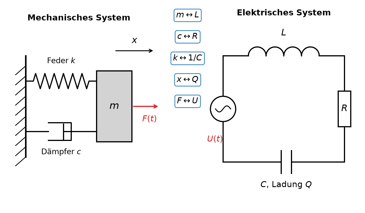
# --- Linke Seite: Feder-Masse-Dämpfer-System ---

# Wand mit Schraffur
ax.plot([0.8, 0.8], [2.0, 6.0], color=col, lw=2)
for y in np.arange(2.0, 6.0, 0.4):
    ax.plot([0.8, 0.4], [y, y - 0.35], color=col, lw=1)

# Feder (Zickzack) von der Wand zur Masse, obere Linie
def feder(ax, x0, x1, y, n=6, h=0.3):
    xs = [x0, x0 + 0.3]
    ys = [y, y]
    dx = (x1 - x0 - 0.6) / (2 * n)
    for i in range(2 * n):
        xs.append(x0 + 0.3 + (i + 0.5) * dx)
        ys.append(y + h if i % 2 == 0 else y - h)
    xs += [x1 - 0.3, x1]
    ys += [y, y]
    ax.plot(xs, ys, color=col, lw=lw)

feder(ax, 0.8, 3.6, 5.0)
ax.text(2.2, 5.7, 'Feder $k$', ha='center', fontsize=10)

# Dämpfer (Zylinder mit Kolben), untere Linie
yd = 3.0
ax.plot([0.8, 1.7], [yd, yd], color=col, lw=lw)            # Stange links
ax.plot([1.7, 2.6, 2.6, 1.7], [yd + 0.35, yd + 0.35, yd - 0.35, yd - 0.35],
        color=col, lw=lw)                                   # offener Zylinder
ax.plot([2.3, 2.3], [yd + 0.3, yd - 0.3], color=col, lw=lw) # Kolben
ax.plot([2.3, 3.6], [yd, yd], color=col, lw=lw)             # Stange rechts
ax.text(2.2, 2.1, 'Dämpfer $c$', ha='center', fontsize=10)

# Masse (Rechteck)
ax.add_patch(plt.Rectangle((3.6, 2.6), 1.4, 2.8, fill=True,
                           facecolor='lightgray', edgecolor=col, lw=lw))
ax.text(4.3, 4.0, '$m$', ha='center', va='center', fontsize=13)

# Koordinate x (Pfeil)
ax.annotate('', xy=(5.9, 6.2), xytext=(4.3, 6.2),
            arrowprops=dict(arrowstyle='->', color=col, lw=1.2))
ax.text(5.1, 6.5, '$x$', ha='center', fontsize=12)

# Externe Kraft F
ax.annotate('', xy=(6.1, 4.0), xytext=(5.0, 4.0),
            arrowprops=dict(arrowstyle='->', color='C3', lw=1.5))
ax.text(5.7, 3.4, '$F(t)$', ha='center', fontsize=11, color='C3')

# --- Rechte Seite: Serien-RLC-Kreis ---
xl, xr, yb, yt = 8.6, 13.4, 1.8, 6.0

# Spule L (obere Kante): Halbkreisbögen
ax.plot([xl, 9.6], [yt, yt], color=col, lw=lw)
theta = np.linspace(0, np.pi, 50)
for i in range(4):
    xc = 9.6 + 0.35 + i * 0.7
    ax.plot(xc + 0.35 * np.cos(theta), yt + 0.35 * np.sin(theta), color=col, lw=lw)
ax.plot([9.6 + 4 * 0.7, xr], [yt, yt], color=col, lw=lw)
ax.text(11.0, 6.8, '$L$', ha='center', fontsize=12)

# Widerstand R (rechte Kante): Rechteck-Symbol
ax.plot([xr, xr], [yt, 4.6], color=col, lw=lw)
ax.add_patch(plt.Rectangle((xr - 0.25, 3.2), 0.5, 1.4, fill=False,
                           edgecolor=col, lw=lw))
ax.plot([xr, xr], [3.2, yb], color=col, lw=lw)
ax.text(xr, 3.9, '$R$', ha='center', va='center', fontsize=12)

# Kondensator C (untere Kante): zwei parallele Platten
ax.plot([xr, 11.3], [yb, yb], color=col, lw=lw)
ax.plot([11.3, 11.3], [yb - 0.45, yb + 0.45], color=col, lw=lw)
ax.plot([10.9, 10.9], [yb - 0.45, yb + 0.45], color=col, lw=lw)
ax.plot([10.9, xl], [yb, yb], color=col, lw=lw)
ax.text(11.1, 0.8, '$C$, Ladung $Q$', ha='center', fontsize=11)

# Spannungsquelle U (linke Kante): Kreis mit ~
ax.plot([xl, xl], [yb, 3.4], color=col, lw=lw)
circ = plt.Circle((xl, 3.9), 0.5, fill=False, edgecolor=col, lw=lw)
ax.add_patch(circ)
ts = np.linspace(-0.3, 0.3, 50)
ax.plot(xl + ts, 3.9 + 0.12 * np.sin(ts / 0.3 * np.pi), color=col, lw=1.2)
ax.plot([xl, xl], [4.4, yt], color=col, lw=lw)
ax.text(8.6, 2.6, '$U(t)$', ha='right', fontsize=11, color='C3')

# --- Zuordnungspfeile in der Mitte ---
pairs = ['$m \\leftrightarrow L$',
         '$c \\leftrightarrow R$',
         '$k \\leftrightarrow 1/C$',
         '$x \\leftrightarrow Q$',
         '$F \\leftrightarrow U$']
for i, p in enumerate(pairs):
    ax.text(7.2, 7.6 - i * 0.85, p, ha='center', va='center', fontsize=11,
            bbox=dict(boxstyle='round,pad=0.25', facecolor='white',
                      edgecolor='C0', alpha=0.9))

ax.text(2.9, 7.4, 'Mechanisches System', ha='center', fontsize=11,
        fontweight='bold')
ax.text(11.0, 7.6, 'Elektrisches System', ha='center', fontsize=11,
        fontweight='bold')

plt.tight_layout()
plt.show()

Abbildung 2: Schema der mechanisch-elektrischen Analogie: Feder-Masse-Dämpfer-System (links) und Serien-RLC-Schwingkreis (rechts) mit der Zuordnung der einander entsprechenden Größen

Mathematische Basis der Analogie

Die Analogie folgt direkt aus der gleichen mathematischen Struktur der Lagrangefunktionen. Für ein mechanisches Feder-Masse-System lautet die Lagrangefunktion: \[ L_{\text{mech}} = \frac{1}{2}m\dot{x}^2 - \frac{1}{2}kx^2 \tag{10}\]

Für einen elektrischen LC-Schaltkreis lautet die Lagrangefunktion: \[ L_{\text{elec}} = \frac{1}{2}L\dot{Q}^2 - \frac{1}{2}\frac{Q^2}{C} \tag{11}\]

Beide Lagrangefunktionen haben exakt dieselbe mathematische Form. Der erste Term ist quadratisch in der Geschwindigkeit beziehungsweise dem Strom, der zweite Term ist quadratisch in der Position beziehungsweise der Ladung.

Die Euler-Lagrange-Gleichungen führen daher auf mathematisch identische Differentialgleichungen. Für das mechanische System erhalten wir: \[ m\ddot{x} + kx = 0 \tag{12}\]

Für das elektrische System ergibt sich: \[ L\ddot{Q} + \frac{Q}{C} = 0 \tag{13}\]

Beide Gleichungen beschreiben harmonische Oszillationen mit derselben mathematischen Struktur.

Praktische Bedeutung der Analogie

Die mechanisch-elektrische Analogie hat weitreichende praktische Bedeutung. Lösungen und Einsichten, die für ein System gewonnen wurden, lassen sich direkt auf das andere System übertragen.

In der Elektrotechnik ermöglicht die Analogie die Verwendung mechanischer Modelle zur Veranschaulichung elektrischer Schaltungen. Umgekehrt können elektrische Netzwerke zur Simulation mechanischer Systeme eingesetzt werden.

Die Analogie geht über einfache Feder-Masse-Systeme und LC-Schaltkreise hinaus. Sie gilt auch für komplexere Systeme mit Dämpfung, externen Kräften und Kopplung zwischen verschiedenen Freiheitsgraden. Die universelle Natur der Lagrangeschen Formulierung garantiert, dass die Analogie auf allen Ebenen der Komplexität erhalten bleibt.

Zusammenfassung

Die Lagrangesche Formulierung der Mechanik bietet einen eleganten und universellen Zugang zur Herleitung von Bewegungsgleichungen. Sie basiert auf dem Hamilton-Prinzip, das die tatsächliche Bewegung als diejenige Trajektorie charakterisiert, die die Wirkung stationär macht.

Die Lagrangefunktion \(L = T^* - V\) fasst die gesamte Dynamik in einer skalaren Funktion zusammen. Aus ihr folgen durch die Euler-Lagrange-Gleichungen die Bewegungsgleichungen des Systems als Differentialgleichungen zweiter Ordnung.

Die Rayleigh-Dissipationsfunktion \(\mathcal{D}\) erweitert den Formalismus auf dissipative Systeme mit Reibung oder Widerstand. Die modifizierten Euler-Lagrange-Gleichungen enthalten dann einen zusätzlichen Term, der die geschwindigkeitsproportionale Dämpfung beschreibt.

Die mechanisch-elektrische Analogie zeigt die tiefe mathematische Verwandtschaft zwischen scheinbar unterschiedlichen physikalischen Systemen. Die Zuordnung \(m \leftrightarrow L\), \(c \leftrightarrow R\) und \(k \leftrightarrow 1/C\) folgt direkt aus der identischen Struktur der Lagrangefunktionen.

Diese universelle Methode ist nicht nur elegant und einsichtig, sondern auch praktisch anwendbar. Sie lässt sich auf beliebig komplexe Systeme mit vielen Freiheitsgraden erweitern und bildet die Grundlage für fortgeschrittene Gebiete der theoretischen Physik wie Feldtheorie, Quantenmechanik und allgemeine Relativitätstheorie. Das Noether-Theorem, das Erhaltungssätze mit Symmetrien der Lagrangefunktion verknüpft, ist ein weiteres mächtiges Resultat, das aus dieser Formulierung folgt.